
Best energy efficiency practices can reduce pump operating costs significantly. This article reviews the basics and presents a new way to account for variation in pump efficiency.
Part 1 (1) of this three-part series reviewed such basics as derivation of the system curve from plant data, the construction of composite performance curves for pump networks, and how to operate and control pumps in parallel to avoid surging and cavitation. This second article discusses how to use variable-frequency drives (VFDs), a subset of variable-speed drives (VSDs), and other energy-efficiency measures such as load management (2) to reduce pump operating costs. It also presents a new way to account for variation in pump efficiency with changing speed when the static head is significant, and uses a natural gas liquid (NGL) pipeline example to explain how the concept works.
Energy requirements (usually electric power) account for nearly 90% of the cost of operating pumps in the chemical process industries (CPI). Assuming 8,400 hr/yr of continuous operation and 72% pump efficiency, the 15-yr cost of operating a typical CPI pump would be as shown in Table 1.
| Table 1. Energy accounts for the largest share of industrial pump costs. | |
| Capital Costs (installed, all inclusive) | 8.5% |
| Maintenance and Repair, including parts and labor | 3.5% |
| Energy (electricity at 6¢/kWh) | 88.0% |

Increasing energy efficiency clearly offers the greatest potential to significantly reduce overall operating costs and improve profits. Brake horsepower (BHP), the actual horsepower delivered to the pump shaft, is:
where Q is the flowrate, ΔP is the pressure drop, and η is the fractional pump efficiency.
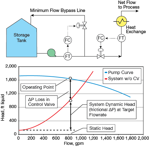
▲Figure 1. In throttling flow control, additional power must be used to offset pressure drop.
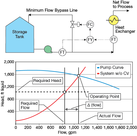
▲Figure 2. Under recirculation flow control, it is necessary to make up for increased flow in the bypass line.
Power consumption can be reduced in three ways — reduce the flow through the pump, reduce the pressure drop in the piping system, or increase the efficiency by operating closer to the pump’s best efficiency point (BEP). The two most common methods of flowrate control are throttling (Figure 1) and recirculation (Figure 2). This control comes at a cost, however. With throttling, the cost is a higher pressure drop, while for recirculation, it is a higher flowrate; both of these require extra power, which ends up heating the fluid.
Improving energy efficiency
On average, approximately 40% of the energy supplied to centrifugal pumps in the CPI is wasted as unrecoverable low-grade heat (Table 2). It is significant that only 6% of energy losses are caused by operational issues, while 34% are built in at the design stage — that is, they are attributable to decisions made during design and the increasingly common practice of fast-tracking this critical step. When inadequate time is budgeted for proper engineering analysis, design engineers are forced to compensate by oversizing pumps, which ensures inefficient operation and can be very costly to undo after production begins.
| Table 2. These five causes account for 40% of wasted energy in pumping. | |
| 1. Low efficiency due to wrong pump choice | 4% |
| 2. Poor installation or maintenance | 3% |
| 3. Low pump efficiency due to wear | 3% |
| 4. Poor system design (piping, valves, etc.) | 10% |
| 5. Poor system control strategy | 20% |
| 40% | |
Fortunately, roughly half of the design-related losses can be reduced by retrofits and a relatively simple revamp of process controls. It is important to recognize that almost no pumping system, whether a single pump or a complex network, regularly operates at its full original design load. As discussed in Part 1, part-load operation (also known as operation at turndown) imposes a huge energy penalty (about 20–30% of total power consumption), most of it in the control valve (CV), or needlessly increases recirculation.
The most effective way to eliminate power loss in individual pumps is to operate each pump at the speed that exactly matches the minimum process flow and head requirements, represented by the system curve. This can only be done by varying operating speed. Several options are available for equipping a pump with variable-speed capability (Table 3).
| Table 3. Pumps can be powered by various types of drivers. | |
| Driver Type | Energy Source |
|---|---|
| Steam Turbine | High-pressure steam exhausting to low pressure |
| Gas Turbine | Fuel |
| Gas Expander | Pressure recovery from high-presure gas |
| Internal Combustion Engine | Fuel |
| Fixed-Speed Motor with Belts | Electricity |
| Fixed-Speed Motor with Gears | Electricity |
| Fixed-Speed Motor with Variable-Frequency Drive | Electricity |
Compensating for oversized pumps
A cheap, but not very efficient, way to compensate for an oversized pump is to trim its impeller diameter, thereby reducing delivered head and the control-valve pressure drop. Care must be taken to retain sufficient flexibility to control flow with a throttling valve, by recirculating excess flow back to the suction tank, or by some other means. The cost is some loss of flow and head capacity.
The pump’s expected flow and head distribution profile determines whether the best results would be achieved by trimming the impeller or by varying the speed. If head variation is ≤ 5% of design and flow variability is ≤ 10% about the mean, impeller trimming may be best option. When pump flow and head both vary widely and unpredictably, however, it is usually best to vary the pump’s operating speed continuously.
The economic feasibility of retrofitting or replacing an existing fixed-speed motor with one that has variable-speed capability depends mainly on the pump’s flowrate distribution profile and the local electric utility’s power rates. As a rule of thumb, variable-speed operation is most feasible when the average flow is less than 60% of the design value.
When the pump drive is a motor, VFDs are usually the most cost-effective retrofit option. For large new installations (>5,000 hp), a direct-coupled steam or gas turbine drive may be a better choice. If the goal is energy savings only (rather than superior process control), depending on the system flow profile, a two-speed motor can cost less than a VFD, offering comparable savings at lower capital cost.
VFDs are generally more desirable than other options, because they also enable exceptionally precise flow control, with minimal lag time between signal input and actuation. A VFD should be thought of as a final control element that replaces the function of the control valve without the accompanying pressure drop. This capability is very important for the pumping of slurries. The energy cost savings are sometimes almost an incidental benefit. Nevertheless, energy savings is VFDs’ most easily quantifiable benefit, and is commonly used to assess economic payback.
The major drawback of VFDs is that they are solid-state electronic devices that must be protected from harsh environmental conditions and exposure to dust, heat, moisture, corrosive gases, etc. If the drives cannot be installed indoors, e.g., inside the motor control center or control room, they must be enclosed in protective cabinets. Lightning protection may also be required for outdoor installations.
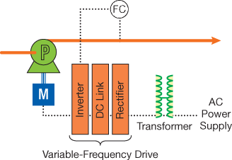
▲Figure 3. Variable-frequency drives (VFDs) must be maintained carefully to protect their sensitive electronic components. Outdoor installations require protective enclosures and may need additional lightning protection.
The principal components of a VFD are the rectifier, the DC link, and the inverter (Figure 3). Depending on the voltage, a transformer may also be required.
Until recently, VFDs were quite expensive, but over the past 10–15 years, advances in solid-state electronics have enabled sharp price reductions, especially in the smaller sizes. The combination of pump and VFD may cost more initially than the pump-plus-CV option, but it has lower lifecycle costs attributable to savings on energy and maintenance (Table 4). An integral unit, suitable for clean environments only, should be considered for new indoor installations or pump replacements of 10 hp or less.
| Table 4. A pump with a variable-frequency drive has lower lifecycle costs than a pump with a control valve. | ||
| Without VFD | With VFD | |
|---|---|---|
| Pump + Motor Purchase Cost | 5 | 6 |
| Variable-Frequency Drive for Motor | 0 | 3 |
| Installation (piping, valves, etc.) | 15 | 18 |
| Operating Power | 55 | 37 |
| Maintenance (parts and labor) | 25 | 16 |
| 100 | 80 | |
It should be emphasized that, at very low operating speeds, numerous mechanical and electrical issues can adversely affect VFD performance. Successful VFD application requires a team effort by the electrical and instrumentation, mechanical, and process engineering departments. Leaving implementation to a single engineer without cross-functional expertise is a recipe for failure.
Using affinity laws to estimate performance
The affinity (or fan) laws (Table 5) can be used to estimate pump performance at off-design conditions. These relationships are based on the assumptions that pump efficiency is independent of speed N (which is mostly true for speeds greater than 50% of the maximum speed) and impeller diameter D (mostly true for diameters greater than 80% of the maximum diameter, Dmax), and that the orginal pump design was close to the BEP. As the impeller diameter is reduced below 0.8Dmax in the same casing, efficiency at the same speed falls off rapidly.
| Table 5. Use the affinity laws to evaluate pump performance at off-design conditions. | ||
| Constant Impeller Diameter | Constant Impeller Speed | |
|---|---|---|
| Capacity |  |  |
| Head |  |  |
| Horsepower |  |  |
| Note: Subscript 1 denotes design conditions and subscript 2 denotes the new condition. | ||
Engineers can use the affinity laws with reasonable confidence to estimate the performance of a pump when the original impeller is trimmed <15%, e.g., when a 12-in. impeller diameter is trimmed to 11 in. or 10.5 in. (Table 6 and Figure 4), based on the pump curve provided by the manufacturer at the time of purchase. Manufacturers’ pump curves should be kept safe and legible, along with the original purchase order documents, in the company library. If any information is missing, difficulties are likely to arise later, especially if the manufacturer has changed the model design or your original contact at the vendor has left the company.
| Table 6. Use the affinity laws to estimate pump curves for different impeller diameters. | |||||
| D = 12 in. | D = 11 in. | D = 10.5 in. | |||
|---|---|---|---|---|---|
| Flow, gpm | Head, ft | Flow, gpm | Head, ft | Flow, gpm | Head, ft |
| 0 | 1,500 | 0 | 1,260 | 0 | 965 |
| 200 | 1,496 | 183 | 1,257 | 160 | 963 |
| 500 | 1,491 | 458 | 1,253 | 401 | 959 |
| 1,000 | 1,470 | 917 | 1,235 | 802 | 946 |
| 1,500 | 1,380 | 1,375 | 1,160 | 1,203 | 888 |
| 2,000 | 1,240 | 1,833 | 1,042 | 1,604 | 798 |
| 2,500 | 1,050 | 2,292 | 882 | 2,005 | 676 |
| 3,000 | 810 | 2,750 | 681 | 2,406 | 521 |
| 3,500 | 520 | 3,208 | 437 | 2,807 | 335 |
| 4,000 | 180 | 3,667 | 151 | 3,208 | 116 |
Would you like to access the complete CEP Article?
No problem. You just have to complete the following steps.
You have completed 0 of 2 steps.
-
Log in
You must be logged in to view this content. Log in now.
-
AIChE Membership
You must be an AIChE member to view this article. Join now.
Copyright Permissions
Would you like to reuse content from CEP Magazine? It’s easy to request permission to reuse content. Simply click here to connect instantly to licensing services, where you can choose from a list of options regarding how you would like to reuse the desired content and complete the transaction.