This article explains some of the core concepts behind pump sizing.
When I left university, I found that I needed additional information to turn my theoretical knowledge of fluid mechanics into the practical knowledge required to specify a pump. Judging by the questions I see asked nearly every week on LinkedIn and elsewhere, I believe this is a problem shared by many engineers early in their careers. This article gives practical insight on how to specify a pump.
Pump types
Pumps can be used to move fluids, which flow from regions of high pressure to regions of low pressure, by increasing the pressure of the fluid. Before you purchase a pump, you must specify the type of pump and make sure it is capable of delivering a given flowrate at a given pressure.
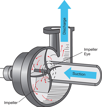
▲Figure 1. In a centrifugal pump, a rotating impeller imparts energy to the liquid moving through the pump.
There are two main pump types: rotodynamic and positive-displacement. In a rotodynamic pump, a rotating impeller imparts energy to the fluid. The most common type of rotodynamic pump is the centrifugal pump (Figure 1). The amount of liquid that passes through the pump is inversely proportional to the pressure at the pump outlet. In other words, the outlet flowrate of a rotodynamic pump varies nonlinearly with pressure.
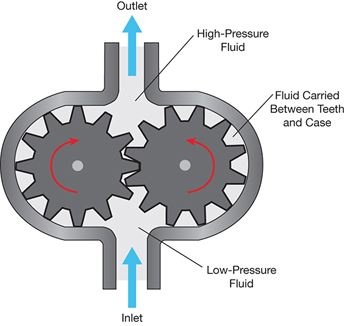
▲Figure 2. A gear pump is a type of positive-displacement pump in which a discrete volume of fluid is trapped and then discharged.
In a positive-displacement (PD) pump, a discrete amount of fluid is trapped, forced through the pump, and discharged. A gear pump is an example of a PD pump (Figure 2). This pumping principle produces a pulsating flow, rather than a smooth flow. Its output flow tends to vary little with respect to the pressure at the pump outlet, because the moving displacement mechanism pushes the slug of liquid out at a constant rate.
Most process pumps are rotodynamic pumps, so you need to know the required outlet pressure to specify the pump that will provide the required flow. Alhough certain system head parameters are calculated the same way whether the driving force for flow is a pump or gravity, this article mainly addresses sizing concerns for rotodynamic pumps.
Pump sizing
Pump sizing involves matching the flow and pressure rating of a pump with the flowrate and pressure required for the process. The mass flowrate of the system is established on the process flow diagram by the mass balance. Achieving this mass flowrate requires a pump that can generate a pressure high enough to overcome the hydraulic resistance of the system of pipes, valves, and so on that the liquid must travel through. This hydraulic resistance is known as the system head.
In other words, the system head is the amount of pressure required to achieve a given flowrate in the system downstream of the pump. The system head is not a fixed quantity — the faster the liquid flows, the higher the system head becomes (for reasons to be discussed later). However, a curve, known as the system curve, can be drawn to show the relationship between flow and hydraulic resistance for a given system.
Pump sizing, then, is the specification of the required outlet pressure of a rotodynamic pump (whose output flow varies nonlinearly with pressure) with a given system head (which varies nonlinearly with flow).
Understanding system head
The system head depends on properties of the system the pump is connected to — these include the static head and the dynamic head of the system.
The static head is created by any vertical columns of liquid attached to the pump and any pressurized systems attached to the pump outlet. The static head exists under static conditions, with the pump switched off, and does not change based on flow. The height of fluid above the pump’s centerline can be determined from the plant layout drawing.
The dynamic head varies dynamically with flowrate (and also with the degree of opening of valves). The dynamic head represents the inefficiency of the system — losses of energy as a result of friction within pipes and fittings and changes of direction. This ineffiency increases with the square of the average velocity of the fluid.
Dynamic head can be further split into two parts. The frictional loss as the liquid moves along lengths of straight pipe is called the straight-run headloss, and the loss as a result of fluid passing through pipe fittings such as bends, valves, and so on is called the fittings headloss.
Fully characterizing a hydraulic system is incredibly complex. Remember that in order to specify a pump, you only need to characterize the system well enough to choose a pump that will perform the job in question. How exact you need to be depends on where in the design process you are. If you are at the conceptual stage, you may be able to avoid specifying the pump at all, but experience suggests that you should use rules of thumb to specify certain parameters (such as superficial velocity) to prevent difficulties later. I also recommend designing the process so that it does not have two-phase flow. Two-phase flow is difficult to predict, and should be avoided in your design if at all possible — head losses can be one thousand times those for single-phase flow. Installing knock-out drums in the system and arranging pipework so that gases are not entrained in liquids can help mitigate two-phase flow.
Superficial velocity is the same as average velocity and is the volumetric flowrate (in m3/sec, for example) divided by the pipe’s internal cross-sectional area (e.g., in m2). A very quick way to start the hydraulic calculations is to use the following superficial velocities:
- pumped water-like fluids: <1.5 m/sec
- gravity-fed water-like fluids: <1 m/sec
- water-like fluids with settleable solids: >1, <1.5 m/sec
- air-like gases: 20 m/sec
Keeping the system within these acceptable ranges of superficial velocities, and avoiding two-phase flow, will typically produce sensible headlosses for the pipe lengths usually found in process plants.
Determining frictional losses through fittings
Dynamic, or friction, head is equal to the sum of the straight-run headloss and the fittings headloss.
The fittings headloss is calculated by what is known as the k-value method. Each type of valve, bend, and tee has a characteristic resistance coefficient, or k value, which can be found in Perry’s Handbook (1) and other sources (Table 1) (2).
| Table1. Each type of pipe fitting has a resistance coefficient, or k value, that can be used to calculate the fittings headloss for the pump system(2). | |
| Fitting Type | k Value |
| Short-radius bends, for every 22.5 deg. allow | 0.2 |
| Long-radius bends, for every 22.5 deg. allow | 0.1 |
| Open isolation valve | 0.4 |
| Open control valve | 10.8 |
| Tee (flow from side branch) | 1.2 |
| Tee (flow straight-through) | 0.1 |
| Swing check non-return valve | 1 |
| Sharp entry | 0.5 |
To use this method, count the number of valves on the piping and instrumentation diagram (P&ID), and the fittings, bends, and tees on the plant layout drawing for the relevant suction or delivery line. Multiply the number of each type of fitting by the corresponding k value, and add the k values for the various types of fittings to get the total k value. Use the total k value to calculate the headloss due to fittings:

where h f is the fittings headloss in meters water gauge (mwg), k is the total k value, v is the superficial velocity (m/sec), and g is the acceleration due to gravity (9.81 m/sec2).
Calculating straight-run headloss
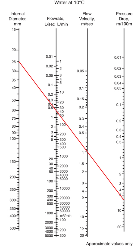
▲Figure 3. A piping nomogram, available from pipe manufacturers, can be used to estimate the straight-run headloss for a pump system. In the example shown by the red line, a 25-mm pipe with a flow velocity of 1 m/sec has a straight-run headloss of about 6 m per 100 m of pipe. Copyright image reproduced courtesy of Durapipe SuperFLO ABS technical data.
At a more-advanced stage of design, you might want to know a pump’s physical size to try out on a plant layout drawing. An easy way to determine the straight-run headloss — the most difficult part of a headloss calculation — is to use a nomogram such as Figure 3 or a table. Pipe manufacturers (and others) produce tables and nomograms that can be used to quickly look up headloss due to friction for liquids.
To use the nomogram, use a ruler to draw a straight line through any pair of known quantities to determine unknown quantities. For example, for a 25-mm nominal-bore pipe with a flow velocity of 1 m/sec, the straight-run headloss is about 6 m per 100 m of pipe. So the headloss through 10 m of this pipe is around 0.6 mwg.
At an early design stage, you often need to calculate the straight-run headloss multiple times. Rather than referring to a table or nomogram numerous times, it can be quicker to set up an Excel spreadsheet and use a formula to calculate the Darcy friction factor and headloss.
Chemical engineering students are usually taught to find the Darcy friction factor using a Moody diagram, which is a summary of a large number of empirical experiments. You can use curve--fitting equations and software such as Excel to approximate the Moody diagram’s output.
Don’t confuse the Darcy friction factor with the Fanning friction factor — the Darcy friction factor is by definition four times the Fanning friction factor. If you do decide to use a Moody diagram to find the friction factor, be aware of which friction factor is on the y-axis.
I prefer the Colebrook-White approximation to calculate the Darcy friction factor. Although it is an approximation, it might be closer to the true experimental value than what the average person can read from a Moody diagram.
The Colebrook-White approximation can be used to estimate the Darcy friction factor (f D) from Reynolds numbers greater than 4,000:

where D h is the hydraulic diameter of the pipe, ε is the surface roughness of the pipe, and Re is the Reynolds number:

where ρ is the density of the fluid, D is the pipe internal diameter, and μ is the fluid dynamic viscosity.
The Colebrook-White approximation can be used iteratively to solve for the Darcy friction factor. The Goal Seek function in Excel does this quickly and easily.
The Darcy-Weisbach equation states that for a pipe of uniform diameter, the pressure loss due to viscous effects (Δp) is proportional to length (L) and can be characterized by:

This iterative approach allows you to calculate straight-run headloss to the degree of accuracy required for virtually any practical application.
I recently came across a paper (3) that suggested there are other equations that provide more accurate results through curve-fitting than the Colebrook-White approximation. If you are producing your own spreadsheet for this purpose, I suggest you look into the Zigrang and Sylvester (4) or Haaland equations (5) (Table 2). These equations also apply for Reynolds numbers greater than 4,000.
| Table 2. These alternative curve-fitting equations can be used in lieu of the Colebrook-White equation to determine the Darcy friction factor. | ||
| Equation | Range | Source |
 | ε = 0.00004–0.05 | (4) |
 | ε = 0.000001–0.05 | (5) |
Adding together the static head, the fittings headloss, and the straight-run headloss will give you the total head the pump needs to generate to overcome resistance and deliver the specified flowrate to the system.
Suction head and net positive suction head
Even at an early stage, I also recommend determining the pump’s required net positive suction head and calculating the net positive suction head (NPSH), as they can affect much more than pump specification. The pump’s required net positive suction head takes into consideration the liquid’s vapor pressure to avoid cavitation in the pump.
I recommend creating an Excel spreadsheet that uses the Antoine equation to estimate the vapor pressure of the liquid at the pump inlet and then calculate the NPSH at that vapor pressure.
The Antoine equation may be expressed as:

where P v is vapor pressure of the liquid at the pump inlet, T is temperature, and A, B, and C are coefficients that can be obtained from the NIST database (http://webbook.nist.gov) among other places. Table 3 shows an example for water.
| Table3. Vapor pressure for water at 30°C, calculated using the Antoine equation. | |||||||
| Material | A | B | C | T,°C | T,K | P v,bar | P v,Pa |
| Water | 5.40221 | 1,838.675 | –31.737 | 30 | 303.15 | 0.042438 | 4,243.81 |
The net positive suction head is:

where P o is the absolute pressure at the suction reservoir, h o is the reservoir liquid level relative to the pump centerline, and h Sf is the headloss due to friction on the suction side of the pump.
Note that NPSH is calculated differently for centrifugal and positive-displacement pumps, and that it varies with pump speed for positive-displacement pumps rather than with pressure as for centrifugal pumps. Equation 6 should only be used with centrifugal pumps.
Determining pump power
After the system head has been calculated, it can be used to calculate an approximate pump power rating for a centrifugal pump:

where P is the pump power (kW), Q is the flowrate (m3/hr), H is the total pump head (m of fluid), and η is the pump efficiency (if you do not know the efficiency, use η = 0.7).
The pump manufacturer provides the precise power ratings and motor size for the pump, but the electrical engineers need an approximate value of this (and pump location) early in the design process to allow them to size the power cables. You should err on the side of caution in this rating calculation (the electrical engineers will be much happier if you come back later to ask for a lower power rating than a higher one).
In certain stages of design development, the preliminary drawings are modified to match likely hydraulic conditions across the design envelope. This may require you to do many approximate hydraulic calculations before the design has settled into a plausible form.
After you have performed the hydraulic calculations, the pump and possibly the pipe sizes might need to be changed, as might the minimum and maximum operating pressures at certain points in the system. As the system design becomes more refined, there might even be a requirement to change from one pump type to another.
Hydraulic networks
The previous sections describe how to calculate the headloss through a single line, but what about the common situation where the process has branched lines, manifolds, and so on? When each branch handles a flow proportional to its headloss, and its headloss is proportional to the flow passing through it, producing an accurate model can become complex very quickly.
My approach to this is to first simplify and then improve the design as much as possible with a few rules of thumb:
- Avoid manifold arrangements that provide a straight-through path from the feed line to a branch. Entry perpendicular to branch direction is preferred.
- Size manifolds such that the superficial velocity never exceeds 1 m/sec at the highest anticipated flowrate.
- Specify progressively smaller manifold diameters to accommodate lower flows to downstream branches.
- Include a small hydraulic restriction in the branch so the branch headloss is 10–100 times the headloss across the manifold.
- Design-in passive flow equalization throughout the piping system wherever possible by making branches hydraulically equivalent.
Perform headloss calculations for each section of the simplified plant design at expected flows to find the flow path with the highest headloss. Use the highest-headloss path to determine the required pump duty — calculate the pump duty at both the average flow with working flow equalization, and at full flow through a single branch. Usually these do not differ much, and the more rigorous answer lies between them. Only if the two results of this approach are very different will I do a more rigorous (and time--consuming) analysis.
If such a rigorous analysis is needed, I create an Excel spreadsheet based on the Hardy Cross method — a method for determining the flow in a pipe network when the flows within the network are unknown but the inputs and outputs are known — and solve for individual pipe flows. Excel’s Solver function can be used to find the change in flow that gives zero loop headloss. In the unlikely event that you have to do this, an explanation of how to carry out the method can be found in Ref. 6. There are many computer programs available to do these calculations.
Pump curves
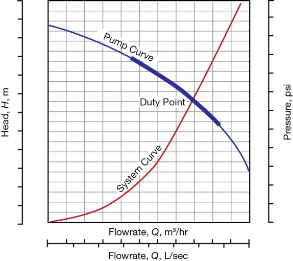
A pump curve is a plot of outlet pressure as a function of flow and is characteristic of a certain pump. The most frequent use of pump curves is in the selection of centrifugal pumps, as the flowrate of these pumps varies dramatically with system pressure. Pump curves are used far less frequently for positive-displacement pumps. A basic pump curve plots the relationship between head and flow for a pump (Figure 4).
On a typical pump curve, flowrate (Q) is on the horizontal axis and head (H) is on the vertical axis. The pump curve shows the measured relationship between these variables, so it is sometimes called a Q/H curve. The intersection of this curve with the vertical axis corresponds to the closed valve head of the pump. These curves are generated by the pump manufacturer under shop test conditions and ideally represent average values for a representative sample of pumps.
A plot of the system head over a range of flowrates, from zero to some value above the maximum required flow, is called the system curve. To generate a system curve, complete the system head calculations for a range of expected process flowrates. System head can be plotted on the same axes as the pump curve. The point at which the system curve and the pump curve intersect is the operating point, or duty point, of the pump.
Remember that a system curve applies to a range of flows at a given system configuration. Throttling a valve in the system will produce a different system curve. If flow through the system will be controlled by opening and closing valves, you need to generate a set of curves that represent expected operating conditions, with a corresponding set of duty points.
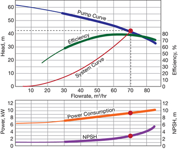
▲Figure 5. Efficiency, power, and net positive suction head can also be plotted on a pump curve. Original image courtesy of Grundfos.
It is common to have efficiency, power, and NPSH plotted on the same graph (Figure 5). Each of these variables requires its own vertical axis. To obtain the pump efficiency at the duty point, draw a line vertically from the duty point to the efficiency curve, and then draw a horizontal line from there to the vertical axis that corresponds to efficiency. Similarly, to obtain the motor power requirement, draw a line down from the duty point to the motor duty curve.
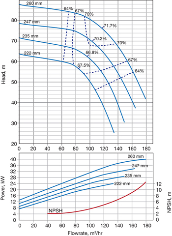
▲Figure 6. A complex pump curve integrates efficiency, NPSH, and impeller diameters on one diagram. Copyright image reproduced courtesy of Grundfos.
More sophisticated curves may include nested curves representing the flow/head relationship at different supply frequencies (i.e., the AC electrical supply’s frequency in Hz) or rotational speeds, with different impellers, or for different fluid densities. Curves for larger impellers or faster rotation lie above curves for smaller impellers or slower rotation, and curves for lower-density fluids lie above curves for higher--density fluids. A more-advanced pump curve might also incorporate impeller diameters and NPSH. Figure 6 depicts pump curves for four different impellers, ranging from 222 mm to 260 mm. Corresponding power curves for each impeller are shown on the bottom of the figure. The dashed lines in Figure 6 are efficiency curves.
These curves can start to look a bit confusing, but the important point to keep in mind is that, just as in the simpler examples, flowrate is always on a common horizontal axis, and the corresponding value on any curve is vertically above or below the duty point.
These more-advanced curves usually incorporate efficiency curves, and these curves define a region of highest efficiency. At the center of this region is the best efficiency point (BEP).
Choose a pump that has an acceptable efficiency across the range of expected operating conditions. Note that we are not necessarily concerned with the entire design envelope — it is not crucial to have high efficiency across all conceivable conditions, just the normal operating range.
The optimal pump for your application will have a BEP close to the duty point. If the duty point is far to the right of a pump curve, well away from the BEP, it is not the right pump for the job.
Even with the most cooperative pump supplier, sometimes the curves that you need to make a pump selection may not be available. This is commonly the case if you want to use an inverter to control pump output based on speed.
However, you can often generate acceptable pump curves using the curves you have and the following approximate pump affinity relationships:


where the subscript 1 designates an initial condition on a known pump curve and subscript 2 is some new condition.
The NPSH relationship in Eq. 11 is more of an approximation than the others. The value of x lies in the range of –2.5 to +1.5, and y in the range of +1.5 to +2.5.
Closing thoughts
These are the basics of pump selection. A final word of advice: If you don’t understand what is presented here, or need to know more, I suggest that you talk to a pump supplier in private. Think twice before you post on social media to ask for advice on the basics of pump selection — the advice you receive may not be correct, and your post may reflect badly on you and your employer.
Literature Cited
- Perry, R. H., and Green, D. W., “Perry’s Chemical Engineers’ Handbook,” 8th Ed., McGraw-Hill, New York, NY, p. 6-18 (2007).
- Moran, S., “An Applied Guide to Process and Plant Design,” Butterworth-Heinemann Oxford, U.K. (2015).
- Genić, S., et al., “A Review of Explicit Approximations of Colebrook’s Equation,” FME Transactions,39, pp. 67–71 (June 2011).
- Zigrang, D. J., and N. D. Sylvester, “Explicit Approximations to the Solution of Colebrook’s Friction Factor Equation,” AIChE Journal,28 (3), pp. 514–515 (May 1982).
- Haaland, S. E., “Simple and Explicit Formulas for the Friction Factor in Turbulent Flow,” Journal of Fluids Engineering,105 (1), pp. 89–90 (1983).
- Huddleston, D., et al., “A Spreadsheet Replacement for Hardy--Cross Piping System Analysis in Undergraduate Hydraulics,” Critical Transitions in Water and Environmental Resources Management, pp. 1–8 (2004).
Nomenclature
A, B, C = Antoine coefficients
D = pipe internal diameter
Dh = hydraulic diameter of the pipe
fD = Darcy friction factor
g = acceleration due to gravity (9.81 m/sec2)
H = total system head
hf = headloss due to fittings in meters water gauge (mwg)
ho = reservoir liquid level relative to the pump centerline
hSf = headloss due to friction on the suction side of the pump
k = resistance coefficient of valves, fittings, bends, tees, etc.
L= length of pipe
NPSH = net positive suction head
P = power (kW)
Pv = vapor pressure of the liquid at the pump inlet
Po = absolute pressure at the suction reservoir
Q = flowrate
Re = Reynolds number
T = temperature
v = superficial velocity
Greek letters
Δp = pressure loss due to viscous effects
ε = surface roughness of the pipe
η = pump efficiency
μ = fluid dynamic viscosity (kg/(m-sec))
ρ = density of fluid (kg/m3)

Copyright Permissions
Would you like to reuse content from CEP Magazine? It’s easy to request permission to reuse content. Simply click here to connect instantly to licensing services, where you can choose from a list of options regarding how you would like to reuse the desired content and complete the transaction.

