
The appropriate values for the proportional, integral, and derivative mode tuning coefficients for a PID controller must reflect the behavior of the process and the desired performance from the control loop.
Tuning a control loop means getting the characteristics of the controller “in tune” with the characteristics of the process. The proportional, integral, and derivative modes each have a tuning coefficient. The objective of tuning is to obtain a value for each of the tuning coefficients.
A major advantage of digital controls over their analog predecessors pertains to the tuning coefficients. In analog implementations, the control engineer specified the tuning coefficients by varying the flow restrictions (pneumatics) or varying the resistors/capacitors (electronics). Most analog controllers had a knob with tick marks for each tuning coefficient. But how accurate were those tick marks? That is, if the gain knob was set to 1.5, what was the actual controller gain? Short of performing tests on the controller (which was rarely done), the answer was elusive. However, with digital controls, if a value of 1.5 is entered for the controller gain, the actual controller gain is exactly 1.5.
Part 1 of this series (CEP, Jan. 2015, pp. 37–44) developed the basic equations for proportional-integral-derivative (PID) control, and presented both differential equations and difference equations. Here, Part 2 explains the tuning coefficient for each mode. Of the three modes, properly tuning the proportional mode is most critical. Hence, the article devotes more explanation to proportional than to integral or derivative.
The role of each mode
This article explains the tuning coefficients used for each mode, but does not explain how to determine values for the tuning coefficients. It does, however, detail a few observations regarding the appropriate role for each mode, and the use of the derivative mode (1). Each mode contributes to the performance of a PID controller.
- Proportional. This mode determines the speed of response for the loop. The higher the controller gain, the faster the loop responds. However, higher controller gains lead to overshoot and oscillations in the response. For each loop, there is a maximum value of the controller gain, known as the ultimate gain, for which the loop is stable.
- Integral. Contrary to popular belief, the integral mode does not produce a faster response. The only contribution of the integral mode is to ensure that the loop can line out only at its setpoint (i.e., there is no droop). It accomplishes this by adjusting the value of the controller output bias (MR). The bias must be changed at a rate consistent with the response characteristics of the process. Changing the bias too rapidly creates more oscillations and, in extreme cases, an unstable loop.
- Derivative. In some applications, derivative reduces the overshoot and oscillations. In turn, this permits a higher value to be used for the controller gain, which increases the speed of response.
Why the emphasis on speed of response? Most processes are slow, some notoriously so. The controls need to make them respond faster.
In practice, there are two choices for mode combinations: PI or PID. The proportional and integral modes are used in all controllers, and derivative is included in a few (on the order of 10%). In the era of pneumatic and electronic controls, a common guideline for ordering controllers was PID for temperature controllers, PI for all others. Today, except for temperature loops, the use of the derivative mode is rare.
The derivative mode projects future values for the process variable by assuming the process follows the current rate of change for one derivative time in the future. Not all processes exhibit such behavior — some make sharp turns. For these, the derivative time must be set to zero.
A good example of an application for the derivative mode is the temperature controller for a jacketed reactor. Two types of jackets are available:
- once-through (Figure 1)
- recirculating, which provides a more uniform temperature throughout the jacket.
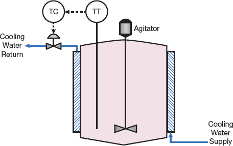
▲ Figure 1. The temperature controller for a once-through jacketed reactor is a good application for the derivative mode.
The derivative mode is almost always used in the reactor temperature controller, regardless of the jacket configuration.
In most production-scale reactors, the reactor temperature responds slowly. The thermal mass (mass times heat capacity) associated with the reacting medium is substantial. A jacket filled with water provides additional thermal mass. As a consequence, if the temperature is increasing by 0.5°C/min, it tends to continue along this path. The rate of increase or decrease changes slowly. The derivative mode can project the current rate of change to estimate future reactor temperatures. A sharp change in the reactor temperature generally indicates that something has gone seriously amiss — beyond the capabilities of the process controls.
This explanation suggests that derivative should be beneficial. Reactor temperatures are very important process variables. Anything that improves the control of the temperature of a reacting medium is music to the ears of the product chemists. Especially in batch applications, closer control of reactor temperatures has become increasingly important. If the instrumentation can deliver tight control, the chemists and process engineers can usually tweak the process to realize benefits such as more uniform product, better yields (which translate into higher production rates), etc.
Derivative is not used in all temperature loops; just in those that matter — such as loops whose performance has a clear and significant impact on process operations. Incidental loops, such as utility temperature loops, are rarely tuned with the derivative mode.
Tuning coefficients
Table 1 presents the options for the tuning coefficient for each mode. The supplier of a commercial control system determines which option is provided. Given the capabilities of digital technology, one would think the supplier would permit the user to make the selection, but that is generally not the case.
| Table 1. Each mode has several tuning coefficient options. | |||
| Control Mode | Tuning Coefficient | Units | Range |
| Proportional | Controller Gain, KC Proportional Band, PB = 100/KC Proportional Gain, KP = KC | %/% % of PV Span %/% | 0.01–99.99 1–9,999 0.01–99.99 |
| Integral | Reset Time, TI Reset Rate, RI = 1/TI Reset Gain, KI = KC/TI | min min–1 (%/%)/min | 0.1–999.9 0.001–9.999 0.1–999.9 |
| Derivative | Derivative Time, TD Derivative Gain, KD = KCTD | min (%/%)-min | 0.00–99.99 0.0–999.99 |
| Note: Some commercial systems use seconds instead of minutes for time. | |||
The implementations in most process controls rely on the PID control equation written as follows:
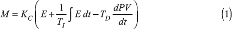
where M is the controller output, E is the control error, TI is the reset time, TD is the derivative time, and PV is the process...
Would you like to access the complete CEP Article?
No problem. You just have to complete the following steps.
You have completed 0 of 2 steps.
-
Log in
You must be logged in to view this content. Log in now.
-
AIChE Membership
You must be an AIChE member to view this article. Join now.
Copyright Permissions
Would you like to reuse content from CEP Magazine? It’s easy to request permission to reuse content. Simply click here to connect instantly to licensing services, where you can choose from a list of options regarding how you would like to reuse the desired content and complete the transaction.