Use Spreadsheets for ChE Problem-Solving

This article will help you improve your Excel spreadsheet skills and will provide you with tools to solve common chemical engineering problems.

Ever since Lotus 1-2-3 and the IBM PC became popular in the early 1980s, chemical engineers have been using spreadsheets for day-to-day problem-solving. This occurred without a major marketing campaign by Lotus Development, which was focused on business applications, and without spreadsheets being included in the formal education of ChEs. This phenomenon speaks loudly to the viability of the spreadsheet, but it also means that chemical engineers often pick up the use of spreadsheets on the fly in a haphazard fashion. Many practitioners miss out on key features and skills in applying the modern versions of the predominant spreadsheet product, Microsoft Excel. This article reviews several useful features of Excel 2013 and techniques for using it.

To be sure, many other software tools — both numerical- and simulation-driven — are available to chemical engineers, especially those employed in larger organizations. Each of these requires a separate learning curve and may be more suitable for calculations associated with larger-scale projects. In many cases, the spreadsheet can be the introduction to these tools. For example, a simpler flowsheet material balance carried out in Excel can produce starting values for a simulator that will enable successful convergence of the flowsheet calculation. Those other software packages, which could cost many thousands of dollars per year in license fees, may be out of reach of chemical engineers in many smaller organizations, who must rely on the ubiquitous spreadsheet for their problem-solving work.

Spreadsheets: Scaling the learning curve

Two features of spreadsheets make them appealing to chemical engineers: their appearance and their function. The row-column layout promotes an organized approach to problem-solving and naturally accommodates tables of data. It is especially convenient for flowsheet material- and energy-balance calculations. Additionally, the answers (the numbers) are displayed in the front while the formulas are in the background. Although many of my faculty colleagues prefer to see the equations and are less concerned with the results, spreadsheets appeal to the practical, upfront nature of the engineer.

The second appealing feature is the “live” calculation nature of the spreadsheet. Change the value in one cell, and any calculations that depend on that cell update auto­matically. This environment allows ChEs to experiment with their calculations and develop an inherent feel for the sensitivity of results to changes in various parameters. This live calculation environment also provides an ideal setting for group interaction where engineers and managers review and brainstorm design and economic calculations to reach decisions.

As chemical engineers increase their skills, their spreadsheets, which normally begin in the upper left-hand corner, tend to expand in both size and content. Consequently, it becomes a challenge to keep the entire content of a large spreadsheet in mind, and, naturally, these larger spreadsheets lack organization and modular design. In the extreme, a large spreadsheet can become barely comprehensible to the author and impenetrable to others. This can create a crisis when the author is no longer available. Unfortunately, in these situations, the spreadsheet must often be jettisoned, and a new author must start over.

Spreadsheets satisfy the need for efficiency and reliability in problem-solving. As chemical engineers learn to use spreadsheets, certain operations become repetitive. Repeating the same action takes time, but learning how to make these operations more efficient will help you save time. Methods to make your spreadsheet more efficient can range from elementary selection techniques to the programming of timesaving macros in VBA (i.e., Visual Basic for Applications, Excel’s companion programming language).

If you allow your spreadsheet to grow incrementally without consideration for organization and modularity, the spreadsheet may become bogged down with embedded errors that are difficult to root out. Or, if you use formulas that are composed primarily of cell address references, your spreadsheet can become very difficult to understand and reverse-engineer. Lack of text documentation in adjacent cells and graphical elements, such as cell formatting, schematic diagrams, well-formatted charts, and embedded typeset equations, exacerbate the difficulty.

Certain features of Excel allow you to solve problems that seem nearly impossible. Learning about these features and incorporating them into your problem-solving activities will increase your capabilities significantly.

The six areas of focus described in this article, taken from a much longer list, can produce immediate results in your spreadsheet work.

1. Use names in lieu of cell addresses

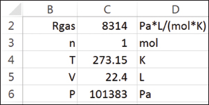
▲Figure 1. For easy readability, this ideal gas law calculation has labels in the left column, values in the center column, and units in the right column.

Consider the ideal gas law calculation in the Excel spreadsheet in Figure 1.

Contrast the following formulas for calculating the value in cell C6:

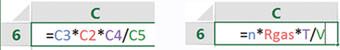
Although this is a simple example, the advantage of the formula on the right is evident. In order to reverse-­engineer formulas that use cell addresses, such as the one on the left, you would have to trace back the source of each quantity. The formula on the right uses cell names that relate to the variable names from the familiar algebraic ideal gas equation. The style of the spreadsheet layout also improves read­ability. In Figure 1, the labels in column B are the same as the names on the cells in column C.

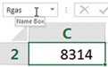
There are three common ways to create names for cells. A convenient method is to select the cell, and type the name into the Name Box field above the column A label:

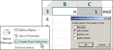
▲Figure 2. Create names for cells using the Create from Selection command.

You can also transfer the label from an adjacent cell onto the cell of interest using Create from Selection in the Defined Names group on the Formula tab of the Ribbon (Figure 2). In fact, more than one label can be transferred with a single command.

Use the Name Manager in the same Defined Names group to create, edit, and delete names. Cell names generally have global scope in the workbook, but it is possible, using the Name Manager, to create names that have scope only in the worksheet where they are created.

Note that certain names are not allowed. First, you cannot create a name that is the same as a cell address. Given the size of the modern worksheet (the Excel spreadsheet has 2¹⁴ = 16,384 columns and 2²⁰ = 1,048,576 rows — a total of 2³⁴ cells), with columns out to XFD, it is easy to confuse a name with a cell address. Second, you cannot use the letters R or C as names or those letters followed by any digits. This restriction harkens back to the R-C method of cell addressing (i.e., row-column), which is rarely used today. Finally, if you transfer labels as names, you will find that in some cases Excel takes editorial license and changes them; for example, the label A(0) becomes the name A_0. For this reason, it is always good practice to check the transferred names before you proceed.

Names can also be defined for rectangular ranges of cells. These names can then be used conveniently in formulas that reference those ranges, such as statistical functions and array formulas.

Names can also be used in VBA code. It is bad practice to use cell addresses in VBA Subs and Functions, because these references will not update in the event any changes are made on the spreadsheet that move the content of these cells.

So, the proverbial bottom line is to use names wherever possible. This raises three additional points:

It is good practice to create a nomenclature table for names, possibly on a separate worksheet. This can be started conveniently using the Paste List command on the Paste Names dialog window. You can access the Paste Names dialog window via the Defined Names group and Use in Formula drop-down list. Your nomenclature list will not be updated automatically, so it is best to generate it as part of the final documentation of a spreadsheet.

When should names not be used? The advantage of cell addresses, both relative and mixed-reference, is in copying formulas and patterns, like index columns, into other cells, for example, using the Autofill feature of Excel, initiated by double-clicking the Fill Handle in the lower right-hand corner of a selected cell. In such cases, the use of cell addresses should be preserved.

If you create formulas that involve cell addresses and later create names for those cells, the names in the formulas will not be automatically updated. You can update the formulas with cell names via the Apply Names dialog window accessed from the drop-down list under Define Name in the Defined Names group (on the Formula tab of the Ribbon).

The use of cell names is especially valuable on larger spreadsheets and even smaller ones that will be used, and hopefully understood, by others.

2. Learn and practice efficient selection, copy, and move techniques

All ChEs should know how to move around the spreadsheet, select blocks of cells, copy cells to other locations, and move cells or blocks of cells. Many of these techniques can be accomplished with the mouse, with the keyboard and the mouse in combination, or using the keyboard alone.

First to consider is moving a selected cell to another location on the spreadsheet. To choose an active cell, click on that cell. The active cell location can be moved quickly to an adjacent cell using the arrow keys. A quick way to jump to a cell far away is to type the cell address or name into the Name Box and press Enter. If a cell name has been defined, you can also use the drop-down list in the Name Box and click on the name there. Another way to do this is with the F5 “Go To” shortcut key.

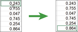
▲Figure 3. Jump to the last cell in a column by double-clicking the lower boundary of the cell selected at the top.

When operating within a column of filled cells, you can jump to the last filled cell in the column by double-clicking the lower boundary of the cell selected at the top (Figure 3). You can also use the same technique to jump across a column of blank cells to a filled cell.

Of course, if a column is short, like the one in Figure 3, you could simply click on the last cell. However, the jump technique is handy for much longer columns (of several hundred cells). As a keyboard alternative, you can use the Ctrl-arrow key combination (Ctrl-↓).

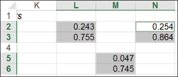
▲Figure 4. To select cells that are not contiguous, hold down the Ctrl key and proceed through selections.

To make block selections rather than jumps, add the Shift key to any of the above techniques. Select an entire block of cells with either the Ctrl-a or Ctrl-* key combination. If you need to select cells or blocks of cells that are not contiguous, you can hold down the Ctrl key and proceed through the selections (Figure 4).

Once cells are selected, you can change their format together, rather than using a tool like the Format Painter and moving from cell to cell. Another application of this technique is to select nonadjacent columns of data to create a chart.

When selecting a lengthy column of data using the Ctrl-Shift-↓ key combination, the bottom of the column is in view with the last cell as the active cell. A neat trick to bring the top of the selection back into view is to press the Tab key followed by the Shift-Tab combination. Of course, you can also drag the slider on the side of the spreadsheet window.

The standard technique for copying cells to adjacent locations is to drag the Fill Handle, located in the lower right corner of the selection. To copy one or more cells to a more distant location, you can initiate the copy with the Ctrl-C key combination, select the destination’s upper left-hand corner cell, and press the Enter key. Alternatively, you can drag the selection to the destination with the Ctrl key pressed; a small + sign will appear adjacent to the mouse cursor arrow when you use this method.

Moving cells is similar to copying cells. To move a cell to an adjacent location, rather than drag the Fill Handle as for copying, you can drag the cell boundary using the arrow cursor. You can also drag selected blocks of cells in that manner. A move can also be initiated with a “cut” shortcut command, Ctrl-X, and terminated with the Enter key, as with the copy technique.

3. Manage units and avoid “magic numbers” in spreadsheet formulas

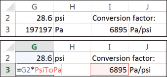
▲Figure 5. Carry out unit conversions in separate cells in your spreadsheet.

Chemical engineers work with a wide variety of engineering units in their day-to-day calculations. Because of this, ChEs are practiced at making calculations consistent when it comes to the units of different variables. This raises the issue of how best to manage conversion of units to a consistent basis for formula-based calculations on spreadsheets. As shown in the ideal gas law example earlier, placing unit labels in adjacent cells is a good practice. And, you should always carry out unit conversions in separate cells on the spreadsheet. Figure 5 shows an example of this in which a pressure is specified in psi but the internal calculations of the spreadsheet require the use of pascals.

Engineers often include unit conversion factors within formulas — this is bad form because it places a number in the formula that may be difficult to understand and interpret. These are sometimes referred to as “magic numbers.” In the spirit of keeping the spreadsheet explicit and easier to analyze and comprehend, avoid putting magic numbers into formulas.

A related tip is to let the spreadsheet carry out the calculations — do not place a number in a cell or formula that is the result of an off-line calculation. For example, it may be tempting to enter one-half a known diameter in a formula that requires a radius. Avoid the temptation and show the divide-by-two calculation explicitly.

In the rush to put a spreadsheet calculation together quickly, we often cut corners, and this comes back to haunt us later. The spreadsheet calculation inevitably expands, and it becomes difficult to interpret formulas that use magic numbers.

4. Set up calculations in their natural sequence and employ targeting methods

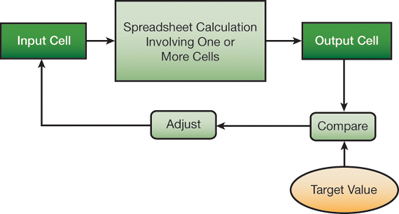
▲Figure 6. Targeting methods, such as Goal Seek or Solver, can help you determine the input value that yields a desired output or target value.

It has been said before many times to start at the beginning and finish at the end. For most chemical engineering problems, there is a natural sequence that starts with basic data and proceeds step-by-step to a final result. However, in many calculations, you may need to find one or more starting values that yield a desired final result, or a target value (Figure 6). The target may be a specific value, or it could be the minimum or maximum of a function, such as cost or profitability. The calculation may have more than one input cell, and there may be constraints on various elements of the calculation.

For one-time solutions of these targeting problems, you can often simply adjust the input value by trial-and-error and meet the target after only a few tries. Excel offers two tools that automate this procedure: Goal Seek and Solver. (The Solver is an add-in provided by Frontline Systems. For information and guidance on using the Solver, see www.solver.com.)

Excel’s Goal Seek is only able to solve target value problems. It is a black-box tool that does not give the user options or control over its numerical procedure. For example, we want to determine the liquid depth in a 4-m-dia. spherical tank that corresponds to a volume of 10 m³. The formula is:

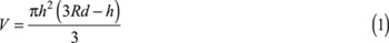
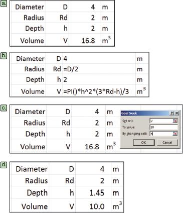
▲Figure 7. The total volume of a liquid in a tank is calculated for an arbitrary liquid height of 2 m (a) by the formulas shown in (b). Use Goal Seek to set the volume equal to 10 m³ by changing cell h (c) to find the depth corresponding to a 10-m³ volume (d).

where V is the volume, h is the liquid depth in the tank, and Rd is the radius of the tank. We set up a calculation on the spreadsheet based on a test value of 2 m for the depth (Figure 7a-b).

Invoke Goal Seek from the What-If Analysis drop-down list in the Data Tools group of the Data tab of the Ribbon. Complete its fields, as shown in Figure 7c, by setting cell V equal to 10 m³ by changing cell h. Upon clicking the OK button and accepting the result, we have the solution that h = 1.45 m (Figure 7d).

The Solver is a more versatile tool that, in addition to solving target value problems, can also solve optimization problems and incorporate constraints. You also have more control of the numerical method used and parameters such as the convergence criterion.

In this example, we use Solver to determine the optimum size of a bin with a cylindrical upper section, a conical lower section, a defined volume, and a minimum bin angle to exceed the angle of repose of the granular material. The optimum is defined as a minimum surface area or area of material used in constructing the bin for a volume of 5 m³.

The required formulas are:

where V_cyl is the volume of the cylindrical upper section, r is the radius, and h_cyl is the height of the cylindrical upper section,

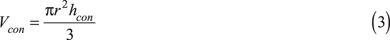
where V_con is the volume of the conical lower section and h_con is the height of the cone,

where V_bin is the bin volume,

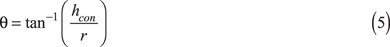
where θ is the conical angle,

where A_cyl is the cylindrical area,

where A_top is the area on the top of the cylinder,

where A_con is the conical area,

where A_bin is the total bin surface area.

The constraints are defined as:

V_bin = 5 m³ and θ ≥ 30 deg. = π/6.

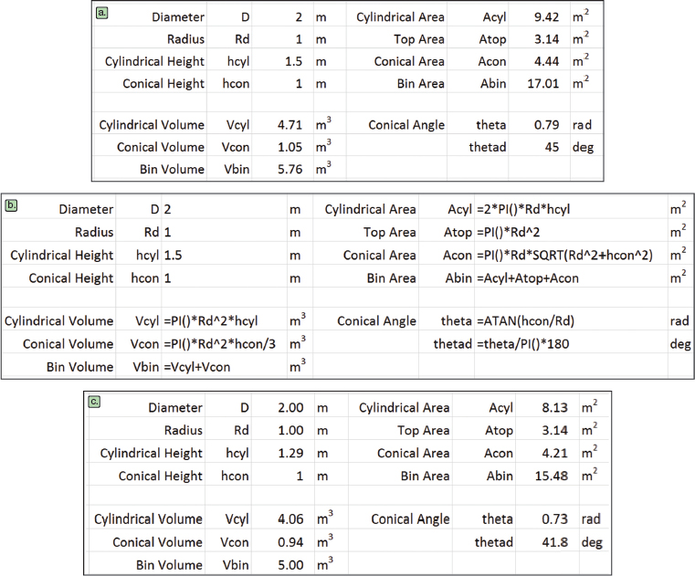
▲Figure 8. To determine the minimum surface area for a bin with a volume of 5 m³ and conical angle of at least 30 deg., the spreadsheet (a) is constructed with the formulas shown in (b). Solver is used to satisfy the constraints and find the minimum value (c).

The starting spreadsheet with a trial calculation is shown in Figure 8a, and the associated formulas are shown in Figure 8b.

The bin volume does not meet the specification of 5 m³ (although the bin angle is greater than 30 deg.). Thus, this is not the optimal solution. Next, specify the Solver Parameters, setting the value of the bin surface area (A_bin) to a minimum by changing the diameter, and the heights of the cylindrical (h_cyl) and conical (h_con) sections. Then, input the constraints:

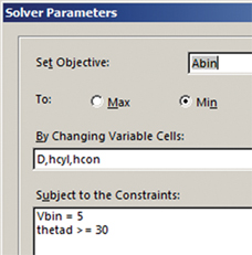
Clicking the Solve button produces the solution in Figure 8c. The bin volume meets the specification of 5 m³, and the angle requirement is easily satisfied. The minimum bin area, and material requirement, is 15.48 m².

Although these are elementary examples, they do demonstrate the importance of setting up calculations in their natural order and using one of the targeting tools to obtain a solution. This is in contrast to reformulating the problem mathematically into one or more nonlinear equations that you would solve, or attempt to solve, using an analytical or numerical method. Although an applied mathematician (or perhaps a ChE faculty member) may prefer to use an analytical or numerical method, using Solver or Goal Seek is more realistic in the world of the practicing ChE.

5. Take advantage of data tables for case studies

Once chemical engineers develop a spreadsheet calculation, however large or small in scale, they are typically interested in running case studies. Case studies can produce results for variations in input values. Engineers very often do this manually, by copying-and-pasting calculation results into an adjacent table and then generating charts to depict the relationships. However, there is a better way.

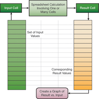
▲Figure 9. Excel’s Data Table tool can tabulate resulting values from a range of input cells.

Figure 9 illustrates the application of Excel’s Data Table tool for a “one-way” case study. A set of input values is mapped into an input cell, and the corresponding values from a result cell are tabulated. This feature is live on the spreadsheet and is implemented with Excel’s TABLE array function.

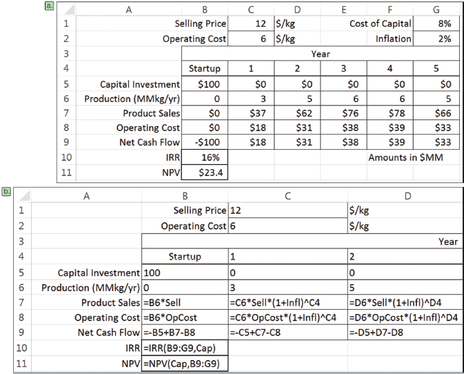
▲Figure 10. This cash flow table (a) uses the formulas in (b) to calculate IRR and NPV.

We can use the Data Table tool to study the cash flow table in Figure 10. In this example, the internal rate of return (IRR) and net present value (NPV) are calculated based on net cash flows in years 0 through 5. The underlying formulas for the first several columns are shown in Figure 10b; the rest follow the established pattern.

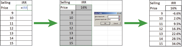
▲Figure 11. You can carry out a case study of IRR vs. selling price using the Data Table command.

To carry out a case study of IRR versus selling price, we set up a column of candidate selling prices and a pointer formula to IRR in the adjacent column, one row up from the selling prices (Figure 11). Then, by invoking the Data Table command from the What-If Analysis drop-down list in the Data Tools group of the Data tab of the Ribbon, and identifying the Column Input cell as the Selling Price (named Sell), we can flesh out the table.

This is a live case study, so when another parameter, such as the inflation rate, is changed, the values update automatically.

The Data Table feature also allows for two-way case studies. To construct a two-way case study, place a column of values for one input parameter on the left of the table and a row of values for a second input parameter in the top row of the table. Then, place the pointer formula, or rule, in the empty cell in the upper left-hand corner of the table.

Excel’s Data Table is a convenient, efficient tool for carrying out case studies using spreadsheets as a calculation engine. Several case studies can be adjoined to a spreadsheet calculation, anticipating questions that might arise about the sensitivity of results to changes in input parameter values. Take advantage of Data Tables!

6. Use Excel’s iterative solver to close recycles and other circular calculations

One of the main reasons chemical engineers became attracted to spreadsheets was for their ability to carry out flowsheet calculations. A process with a recycle stream involves a circular calculation that cannot proceed automatically because of its iterative nature. In a more general sense, many process calculations, when laid out in logical sequence, involve circular calculations.

In such a situation, a value is needed to continue the calculation, but that value is calculated later in the scheme. The strategy for solving such calculations is to specify a starting value and then “recycle” the value calculated later until the loop converges. It is possible in some cases to reformulate this problem mathematically to eliminate the circular calculation, but that leaves the scheme in an unnatural format that is more difficult to manage and understand.

Circular calculations that use a simple substitution method do not always converge, but in chemical engineering problem-solving they commonly do converge. For cases of nonconvergence, numerical methods are available, notably that of Wegstein, that may force convergence.

I suggest taking advantage of Excel’s Iterative Solver to converge circular calculations. As a simple example, we can use the Colebrook equation relating the Moody friction factor (f_M), Reynolds number (Re), pipe inside diameter (D_i), and pipe roughness (ε) for turbulent flow:

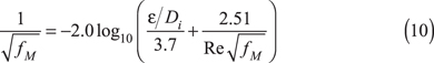
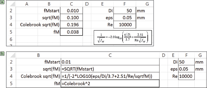
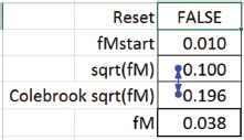
▲Figure 12. To calculate the Moody friction factor, an iterative calculation must be used (a). The underlying formulas (b) show how the starting f_M value will be different than the final f_M value.

Notice that in order to compute f_M, we need a value of f_M for the right-hand side of Eq. 10. Therefore, a simple, analytical solution is not available. So, a circular calculation arises. Figure 12a is a spreadsheet that arranges this calculation, with the underlying formulas shown in Figure 12b.

This calculation has not converged because the sqrt(f_M) does not equal the Colebrook sqrt(f_M). So, we expand the spreadsheet to include the option to “close the loop” by a modification of the sqrt(f_M) formula:

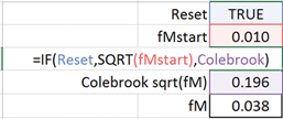
Now, when Reset is FALSE, the loop is closed. However, Excel complains that there is a circular path:

To resolve this, set up the Iterative Solver via File ⇒ Options ⇒ Formulas:

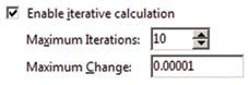
The Maximum Iterations was set to 10 because, based on our experience with manual recalculation, this guarantees convergence of the circular calculation to the desired precision. The result is:

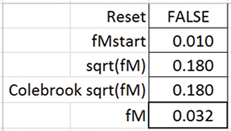
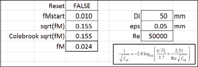
▲Figure 13. The iterative solver will update automatically if any initial parameters, such as the Reynolds number, are changed.

The calculation also updates automatically if another parameter is changed, such as setting Re = 50,000 (Figure 13). So, as circular calculations arise in your chemical engineering problem-solving, embrace them and manage them with the Iterative Solver.

Some additional tips

It would be possible to elaborate on many more topics of interest to ChEs here, but space and time are limited. So, to conclude, we will mention in rapid fashion other considerations. These are dealt with in numerous references and in short courses offered through the AIChE Academy.

Consider using array formulas instead of copying formulas with relative addresses. A single array formula can replace many formulas that were generated, for example, by copying a formula down a column adjacent to other columns of data. Array formulas also allow for matrix calculations (transpose, multiply, inverse, determinant). They are inserted using the Ctrl-Shift-Enter key combination instead of just the Enter key.

Use templates to streamline chart creation. Creating charts can be a time-consuming activity in Excel.

Embed schematic drawings and typeset equations. Schematic drawings, created with such software tools as PowerPoint and Visio, can be copied and pasted into Excel workbooks. In addition, typeset equations, such as the Colebrook equation shown in Figure 12, can be embedded as objects (e.g., Insert ⇒ Text ⇒ Object ⇒ Microsoft Equation 3.0). These aid greatly in the understanding of spreadsheet calculations.

Modularize workbooks into separate worksheets and design individual worksheets with diagonal blocks. Don’t allow your spreadsheets to grow in an amorphous, dis­organized fashion. Calculations should be divided into modules that can be arranged on separate worksheets. Larger calculations on a single worksheet should be segmented into diagonal blocks to allow the row heights and column widths of those blocks to be adjusted independently for readability, and so each block can be reached quickly via a name associated with its upper left-hand corner.

Wade cautiously into VBA by recording time-saving macros. Developing skill and expertise in VBA programming for Excel is a big step to take. However, you can get a big return for a small investment by recording macros that replace a multistep procedure on the spreadsheet with a single shortcut command. Since Excel/VBA writes the macro after recording your actions, you can readily make modifications to the VBA code generated in the Visual Basic Editor (Alt-F11 to get there and back). This is facilitated because VBA code is verbose and easy to read but difficult to compose.

Consider user-defined VBA functions for standard engineering calculations and special needs on the spreadsheet. Engineering formulas can be packaged into convenient user-defined VBA functions, which allow you to efficiently and reliably implement the formulas. This is a bit more difficult than recording macros, but it is still possible with some practice. You can also package a collection of user-defined VBA functions into an Excel Add-In.

The topics reviewed in this article may help you improve your spreadsheet knowledge. The article is by no means comprehensive but may fill out a few gaps in your abilities with Excel.

Happy spreadsheeting!

This article is based on the AIChE online course, “Spreadsheet Problem-­Solving for Chemical Engineers.” To register for this course, or to watch a webinar presented by David Clough, visit www.aiche.org/academy.