
Sections
Good process control requires more than just correctly tuning the controller. First, you need to understand the parts of the process to determine the necessary type of control.
University control courses typically concentrate on the mathematical complexities involved in modeling a control system, but they do not spend much time on the actual equipment used to do the controlling (1). While I learned about transfer functions, LaPlace transforms, and other technical details in school, when I got my first job, I did not even know how a proportional-integral-derivative (PID) controller worked! In my case, I learned the basics from an instruction manual for a pneumatic controller.
Good process control requires more than just correctly tuning the controller. It is critical to first understand the interactions between the parts of the process to decide what type of control is needed. This article describes how process equipment can impact process control, the external factors that affect controller tuning, and the types of tuning that can be implemented.
Equipment problems can affect process control
Tuning a system that is being used for the first time requires a lot of experience. Typically, if a control system is being designed for a new process, the design team will specify a standard PID control loop and rely on experienced control engineers to do the initial tuning. The methods described in this article apply only to a system that is already in operation.
Identifying a loop with control problems is usually easy. Most of the time, you can simply look at the process plots in the control room and pinpoint the ones that are chasing a setpoint or cycling (Figure 1). Issues related to hardware and system configuration, which are critical to good control, may be at the root of these control issues. This section describes some of the problems that can be caused by hardware and system configurations. The examples below assume that a liquid flow is being controlled by a valve.
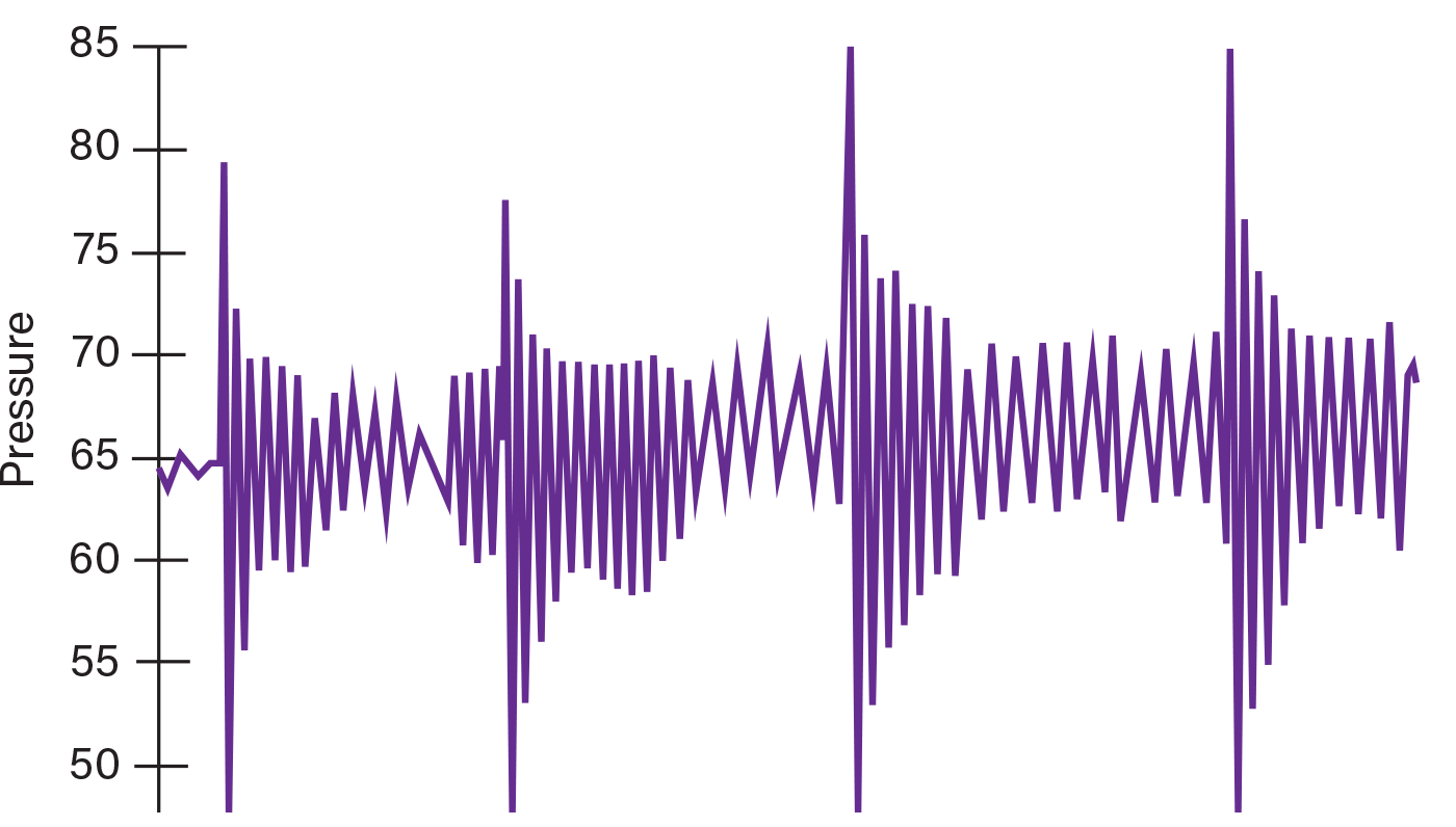
▲Figure 1. This process plot shows pressure cycling in a stripping column.
Oversized valves. If a valve is too large for the process, more fluid than is needed will pass through the valve as the controller opens it, increasing the flowrate past the setpoint. As a result, the controller will then close the valve. As the flowrate decreases past the setpoint, the controller will start to open the valve again. The flow will then shoot up once more and the controller will again close the valve. This action creates a kind of on-and-off control that produces a series of bumps in the valve plot.
Figure 2 is a process plot for a system that needs at least 42 ft3/hr of steam to achieve the desired liquid temperature at the exit of a heat exchanger. When the flowrate approaches 42 ft3/hr, the temperature approaches its setpoint and the controller begins to open the valve to maintain the liquid temperature. However, the valve is oversized, so when it is just 8% open, too much steam flows into the exchanger. The temperature rapidly increases and the valve closes. When the liquid’s exit temperature begins to fall, the cycle repeats.
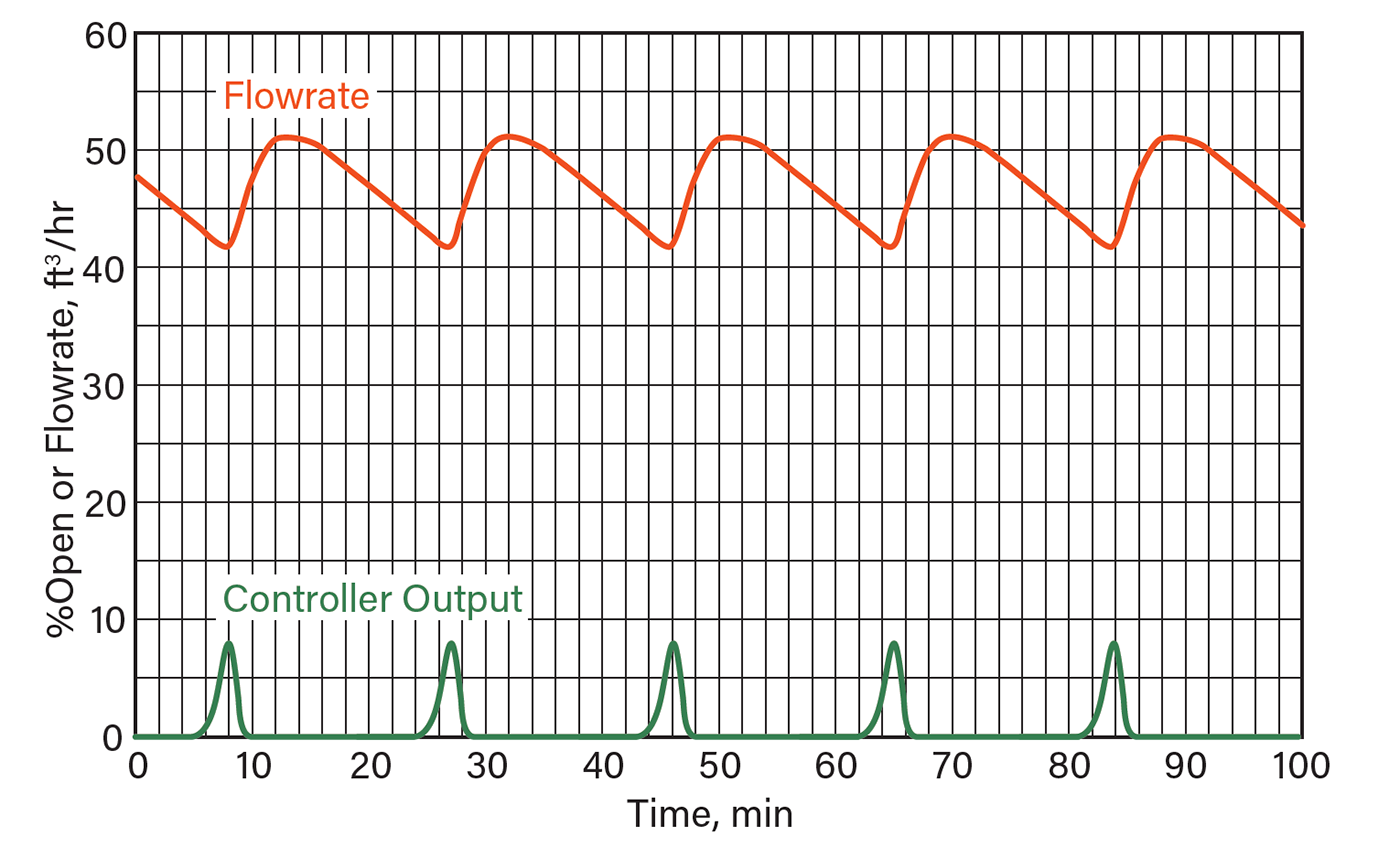
▲Figure 2. If a valve is oversized, too much fluid will pass through it as the valve opens, which will trigger the controller to close the valve. The flow will cycle up and down as it tries to achieve the setpoint.
Even if the valve does not close completely but operates at less than 20% open, the valve gain (i.e., change in output/change in input) will be large, which will cause a large change in the process variable (PV) for a small change in the controller output (OP). For example, opening the valve from 50% to 51% is a change of only 2% of the valve setting. Increasing the valve from 20% to 21% is a change of 5% of the valve setting. This larger gain will make the controller’s job more difficult, because it has to control the output more precisely.
To function properly, valves should be sized to be 30–70% open during normal operation. This value depends on the range of flowrates needed by the process. If the desired operational flowrate is always the same (i.e., no changes in production rate), the valve could be sized to operate at 70–80% open under normal conditions. This design will enable selection of the smallest and cheapest valve for the application.
Hysteresis. When valve opening or closing lags behind the signal and the valve position ends up in a different place than intended, it is called hysteresis. If a valve that produces 100 gal/min of flow at 50% open is opened to 60% and then lowered back to 50%, it should give a flow of 100 gal/min again. If, for example, it now produces 105 gal/min, the valve is suffering from hysteresis.
The amount of hysteresis that occurs in the valve is called its deadband. Sometimes deadband can be lowered by tightening the linkage between the valve stem and the actuator. But if the hysteresis cannot be corrected mechanically, a valve positioner may be needed. Valve positioners act as a mini control system for the valve, measuring the position of the valve stem and adjusting the actuating pressure to move the valve to the desired location. A standard valve actuator (i.e., without a positioner) adjusts the actuating pressure to a set value and assumes that the valve will reach the desired location.
Hysteresis can also be overcome by the integral function in a PID controller, which continues to move the valve in the desired direction until the setpoint flow is reached.
Stiction. Valves may stick as they open and close; this is called stiction. As the signal increases, the valve does not move until the pressure is high enough to overcome the resistance. When it does, the valve jumps to the new position. Then, as the signal decreases, the valve sticks again until the pressure is low enough that it jumps in the opposite direction. This often occurs in valves with packed stems when the packing is compressed too tightly.
If the stiction is severe, it will produce a series of steps in the plot of the actual flow as the valve suddenly opens or closes to jump to the new position. In many cases, stiction is not severe enough as to produce this stepwise pattern. Instead, valves stick in a position until the controller applies enough pressure that the valve suddenly moves. The valve is typically then able to move around well until the controller stops moving it and it sticks again (Figure 3).
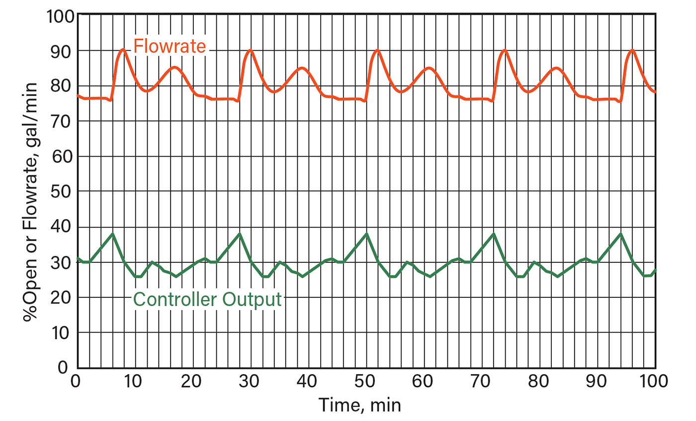
▲Figure 3. If stiction is severe, it produces a step pattern in the process flow plot. However, it more often produces the pattern of peaks and valleys shown here as the valve sticks, overcomes the resistance, moves easily, and then sticks again.
In the plot in Figure 3, the flow is initially about 77 gal/min and falling, but the controller wants the flow to increase to 79 gal/min. Starting at two minutes, the controller increases the output to the valve from 30% to 38% and nothing happens. Then, the valve stem breaks loose from the grip of the packing and opens to 38%, which suddenly increases the flow from 75 gal/min to 90 gal/min. The controller immediately starts trying to close the valve to get the flow back below 80 gal/min. The unstuck valve is able to move freely in response to the controller, bringing the flow back down to around 75 gal/min. The valve stops moving and becomes stuck when it is about 30% open at 23 min. The controller starts trying to open the valve once more and the cycle repeats.
To identify if stiction is a problem, look for a sudden increase in the flowrate after the OP has been increasing for a while. If an increase in OP causes the flowrate to increase slowly, the problem is just a long response time in the control loop, even if the flowrate initially does not respond for several minutes. If the flowrate remains unchanged for several minutes and then suddenly increases, the problem is a sticking valve.
A valve suffering from stiction is difficult to tune and usually requires a mechanical solution if the amount of variation it produces is a problem for the process. Lubricating the valve stem may eliminate stiction. Slightly loosening the nut that confines the packing to reduce the pressure on the stem may also work, but the valve needs to be monitored to ensure there is no leakage around the stem.
Wrong valve type. The three main types of control valves include quick-opening, linear, and equal-percentage valves (Figure 4). Quick-opening valves provide a large opening at low signal values; at higher signal values, the opening size increases more slowly. Equal-percentage valves do the opposite — they provide a small opening at low signal values, and as the signal increases, the opening size increases more quickly. Linear valves open in proportion to the signal value throughout the range.
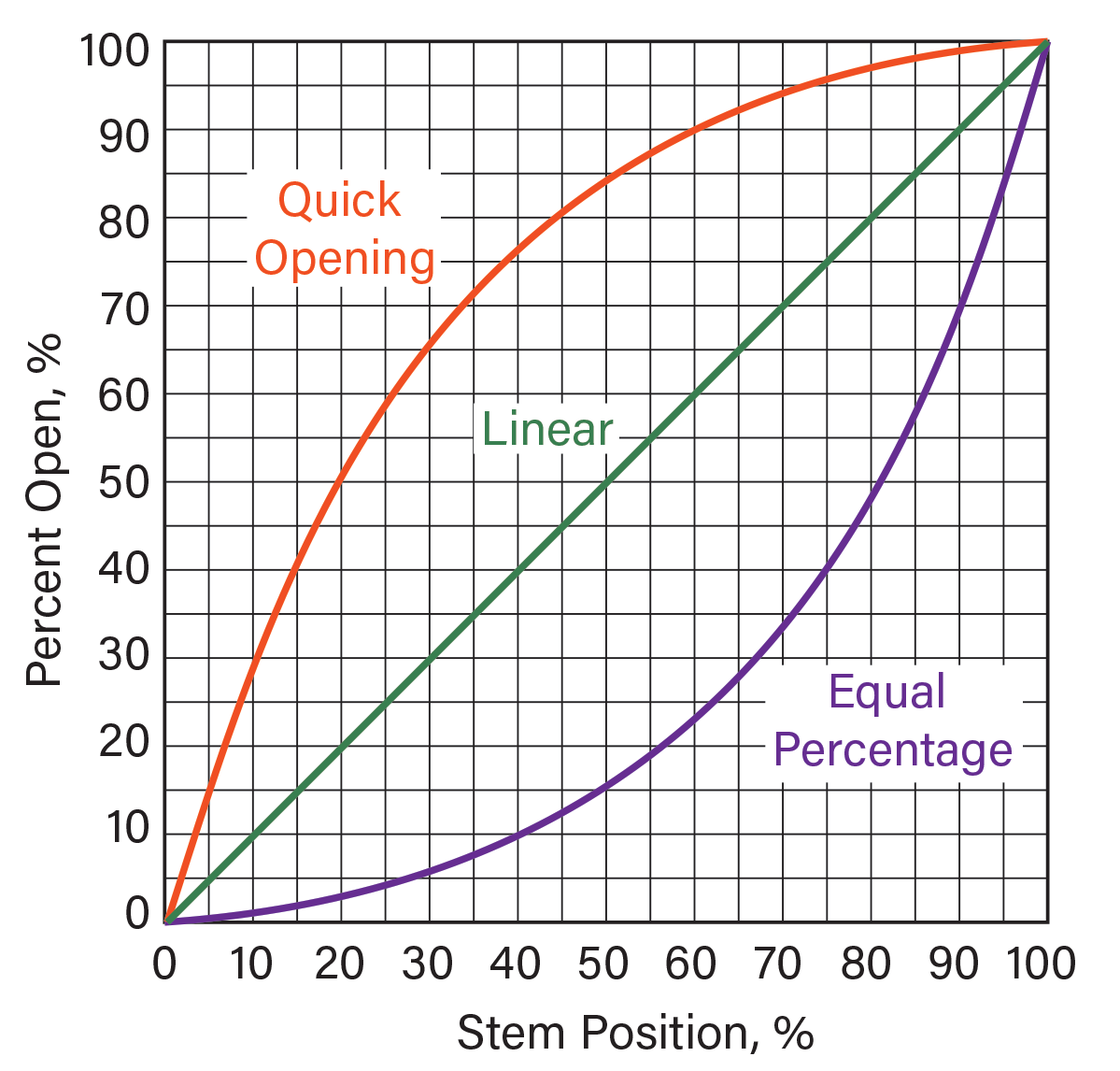
▲Figure 4. These plots show the idealized function of quick-opening, equal-percentage, and linear control valves.
If a quick-opening valve is run at 25% open, control will be difficult because a small change in the valve position will produce a large change in the flow. The ideal quick-opening valve controls best in the range of 40–70% open. The ideal equal-percentage valve controls best in the range of 30–60% open. These types of valves are suitable for applications where you might need many times the normal flow in an emergency. For example, the equal-percentage valve could be used to control the temperature of a reactor. The valve might normally operate at 30% open, but if the temperature starts to rapidly increase, the valve can be opened to 70%, providing a high flowrate of cooling water to the jacket to lower the reactor’s temperature.
Linear valves provide good control across a broad range of flows. They are suitable for systems that need to operate at a range of production rates.
Interactions between pumps and valves. There are many different types of pumps. Some are positive displacement pumps, such as lobe, tube, and piston pumps. Others are centrifugal pumps, which spin the liquid around in a chamber to create the pressure needed to make it flow through a pipe. Centrifugal pumps present a special kind of problem for control systems because as the flow increases, the driving pressure that provides the flow decreases (Figure 5).
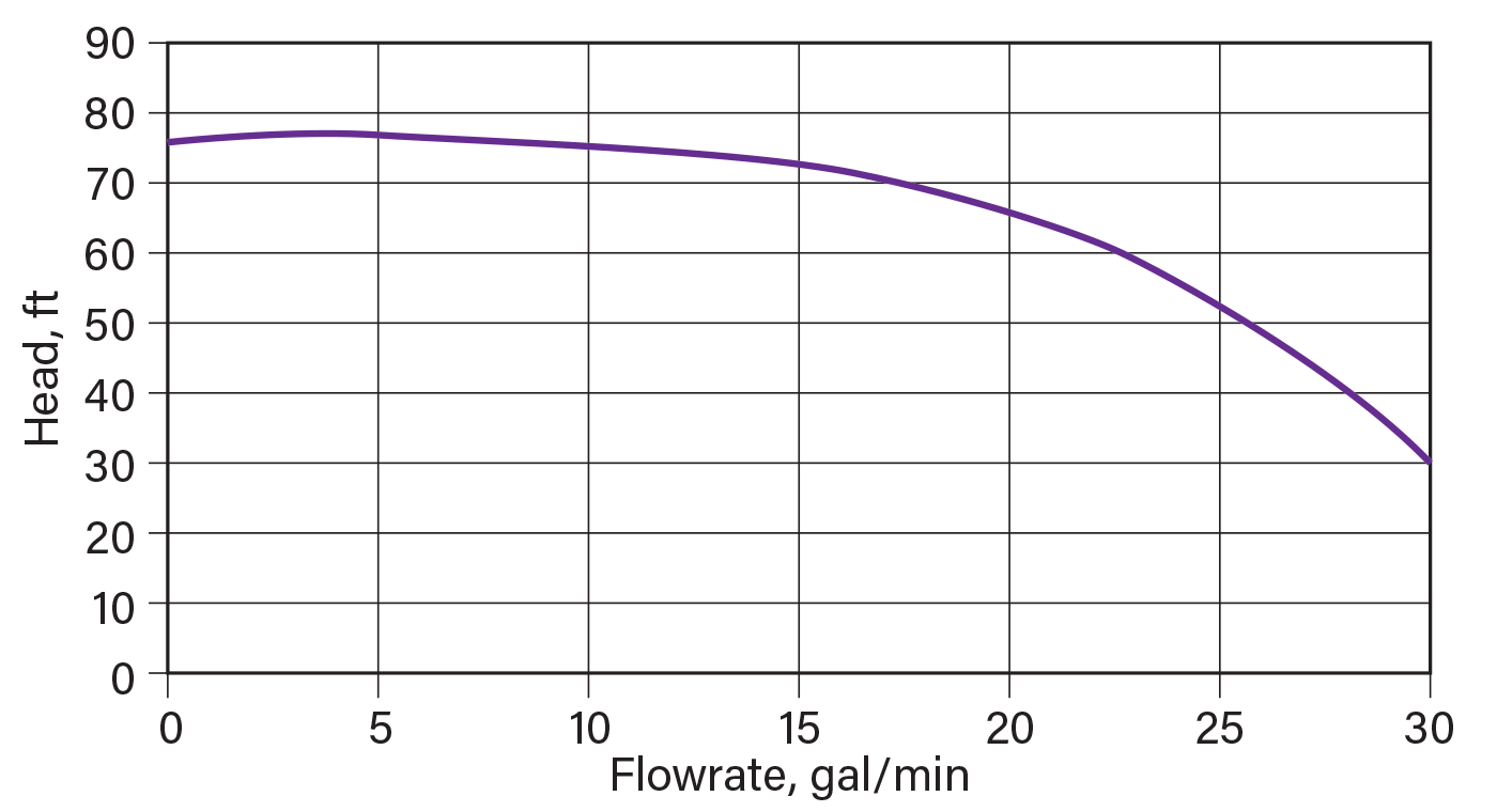
▲Figure 5. This typical head vs. flowrate curve for a centrifugal pump illustrates that at high flowrates the achievable head drops off.
Consider a process that requires a flowrate of 20 gal/min and the pressure in the pipe is 30 psig. A valve could be sized to achieve this flowrate with a pressure drop of 15 psi (i.e., half of the line pressure) at 50% open. This seems reasonable, but if a centrifugal pump provides the pressure to drive the flow, it may not be able to achieve the higher flowrates required during upsets (e.g., startups, shutdowns, changes in production rate). Assume that the 30 psig pressure is equal to a head of about 66 ft of liquid. The pump generates lower head pressures at higher flowrates. Therefore, opening the valve to increase the flowrate from 20 gal/min to 25 gal/min would lower the available head from 66 ft to 53 ft — a decrease of 20%. If the valve has to operate at 90–100% open to achieve the desired flowrate, the process will be very difficult to control.
A large, equal-percentage valve with a low pressure drop would be an appropriate valve for this service because the increasing rate at which this valve opens would help to offset the decreasing pressure provided by the pump. For an existing system, the control issues could be addressed by recommending a larger valve trim or a larger impeller for the pump. Modifying the pump with a larger impeller would flatten the pump curve at 20 gal/min and could help to stabilize operation. However, this will likely increase energy costs, as centrifugal pumps typically operate most efficiently in the region to the right of the flat portion of the head curve.
Look for external causes first
When a piece of equipment has control problems, first examine the inputs to the system. Control problems in a column or reactor could be due to problems upstream. If, for example, the feed to a column or the flow of steam to the reboiler is fluctuating, then the control system cannot find a good control point and will always be searching for a solution. Look for variations in the feed rate, feed composition, feed temperature, system pressure, steam pressure, chilled water temperature, etc. These external variations may be causing the problem, so they should be addressed first. Once the upstream variations are fixed, the control problem in the column or reactor may resolve itself.
In one system that I tuned, I found that an entire section of the process seemed to have control problems that caused cycling. I traced it to a column that had a steam load and tray temperature that were constantly oscillating. I checked the inputs to the column and found that the feed rate varied significantly. I traced the feed flow variation back to a surge tank that was collecting the bottoms from a stripping column further upstream.
The level in the tank was being tightly controlled at 50%, but there was no reason that it had to be held at precisely that level. The level could vary as long as the tank did not empty out or overflow. I loosened the level control on the tank to allow the level to vary between 40% and 60%. The valve would now only make small adjustments as the level rose or fell, which allowed us to smooth out the variations in the tank’s discharge flowrate and eliminate the big swings in the column’s feed flowrate. Once the feed to the column was steady, the control problems were eliminated and the cycling issues downstream were solved.
Another source of control problems is the setup of the control system itself. Some equipment may have two or more control systems. Distillation columns, for example, typically have a control on the reflux ratio and on the reboiler heat load (2, 3). The reflux ratio is adjusted to control the temperature on an upper tray to meet an overhead purity specification, and the reboiler is adjusted to control the temperature on a lower tray to meet a bottoms specification.
This control scheme sounds good in theory, but it creates a system where the two controllers are fighting each other. If the upper temperature gets too high, the reflux ratio increases to send more of the low-boiling component back down the column to reduce the temperature. This puts more load on the bottom of the column and causes the temperature of the lower trays to decrease. The reboiler control system responds by increasing the boilup and sending more of the high-boiling component back up the column. This increases the temperature of the upper trays and the cycle starts again.
To settle this fight between the two controllers, decide which output is most important. Is it more critical to keep the high-boiling component out of the distillate or to keep the low-boiling component out of the bottoms? If keeping the low boiler out of the bottoms is more important, then keep the bottoms temperature controller as-is and loosely tune the reflux ratio controller. The bottom will hold its specification and allow the top temperature to hover around the setpoint. Any variation in the composition will be evident in the distillate. When this control method was applied to an actual column, it allowed good automatic control of a system that was so unstable it had been run manually for years.
What type of control do you need?
Most people who tune a controller or use a control program to do the tuning assume that the objective is to achieve rapid response on a single device. But this is not always the case. There are four basic types of control:
- Rapid response allows the process to vary but attempts to bring the PV back to the setpoint within a short period of time.
- Slow response can help solve operational issues. A piece of equipment can be set to have loose control, such as the level of the surge tank described in the previous section, which allows the equipment to absorb upstream variations.
- Hybrid response, also called cascade control, is used when a control variable that is manipulated to affect a process value (e.g., temperature, pressure, flowrate) has a variable source. Cascade control can be effective, for example, if steam is used to control a process temperature, but the flowrate of steam from the header varies due to variable header pressure. A main loop reads the temperature and decides how much steam is needed. It then sends this information to a secondary loop that regulates the steam flow. The secondary loop has a rapid response and the main loop has a slow response.
- Tight control may be needed when small deviations in parameters like pH or temperature can cause product loss or dangerous conditions. The emphasis is not on minimizing the time of the response but on minimizing the amount of variation from the setpoint. Usually, increasing the proportional and integral control parameter values can achieve the necessary level of control response. (Derivative control is sometimes used for tight control, but it is a more complex procedure and is not covered in this article.)
More advanced control schemes can be developed that involve material or energy balances around a piece of equipment or a part of the process. This is necessary in certain instances, such as to estimate the amount of unreacted raw material accumulating in a reactor to avoid a runaway reaction. However, such control schemes should not be implemented if a simpler control strategy will work. Complex systems require that all of the sensors work properly. If one temperature or flowrate sensor drifts, the whole system becomes unreliable because the material or energy balance will be inaccurate.
On the other hand, if a temperature or flow sensor drifts in a simple PID system, the setpoint can be lowered or raised in that part of the system and the rest of the process can continue to run until repairs can be made. If a sensor malfunctions completely, the PID system can be run on manual until it can be repaired. Simple systems are more rugged, and with proper tuning, PID systems can control almost any process.
In closing
This article describes some of the items that can cause control problems, the types of control that are available, and some actions to take before starting to tune.
In an article to follow, I will describe the basics of the PID controller and two different methods that can be used to tune the controls for live systems.
Literature Cited
- Alford, J., and G. Buckbee, “Industrial Process Control Systems: A New Approach to Education,” Chemical Engineering Progress, 16 (12), pp. 35–42 (Dec. 2020).
- Herzog, C., “Develop Distillation Controls During Process Design,” Chemical Engineering Progress, 17 (2), pp. 31–37 (Feb. 2021).
- Taube, M. A., et al., “Achieve the Benefits of Intensification through Process Control,” Chemical Engineering Progress, 17 (3), pp. 44–49 (Mar. 2021).

Copyright Permissions
Would you like to reuse content from CEP Magazine? It’s easy to request permission to reuse content. Simply click here to connect instantly to licensing services, where you can choose from a list of options regarding how you would like to reuse the desired content and complete the transaction.