Analyzing the Performance of Pump Networks Part 1: Basic Theory

This article demonstrates how to construct a pump’s system curve and explains the four most common mistakes encountered when operating centrifugal pump networks.

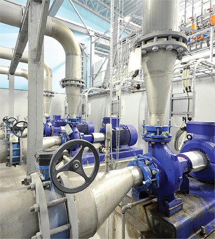
▲Figure 1. Centrifugal pump installations are very common in the chemical process industries (CPI).

Centrifugal pumps are among the most ubiquitous items of process equipment in the chemical process industries (CPI) (Figure 1).

The fraction of electrical power consumed by pumps at typical plant sites in the U.S. and Canada has been reported in the literature to be between 70% and 90%. However, pumps and compressors that are driven by steam turbines or other non-electric prime movers consume much less electrical energy. Although there are many different types of pumps, the vast majority (around 90%) of installed pumps in the CPI are centrifugal pumps.

The dominant 20-yr lifecycle costs associated with the average pumping application in the U.S. are electric power and maintenance, with power accounting for 55% of the total and maintenance making up 25%. Initial capital costs typically account for about 20% of the total; the purchase cost of the pump/motor assembly accounts for around one-fourth of that, or only 5% of the total.

The lifecycle costs for larger installations in the CPI that run continuously are even more heavily weighted toward energy. Therefore, it makes sense to choose a pumping system for high efficiency, reliability, and ease of maintenance. Nonetheless, the prevailing industry practice is to make the purchasing decision on the basis of lowest first cost. Hopefully that will change if companies modernize their procurement procedures.

This is the first of a three-part series that reviews the basic theory of pump hydraulics and gives practical tips from the authors’ collective experience from a wide range of industries on how to design, operate, control, and troubleshoot pumping systems in complex applications.

The series addresses four main topics:

• construction of the system curve from plant data
• construction of composite curves for pump networks
• proper operation and control of pumps in parallel to avoid surging and cavitation
• use of variable-frequency drives (VFDs) and load management techniques to save energy.

This article, Part 1, focuses on the first three bullet points. Parts 2 and 3 will address the issue of energy efficiency improvement through the use of better control methods and VFDs. The lessons highlighted in the articles apply equally to all pumping applications regardless of the industry.

Basic theory

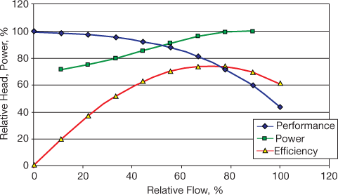
▲Figure 2. The principal curves that define a pump’s operating characteristics are the performance curve (blue), the power curve (green), and the efficiency curve (red).

The relationship between head and flowrate for a single pump is called its characteristic curve or performance curve (Figure 2). The manufacturer or vendor will provide the pump’s performance, efficiency, and power curves at the time of purchase, and the original copy should be maintained securely in the company library or archives (not in the control room). Because it is common for pump models to be discontinued or for vendors to go out of business, pump curves are very difficult to retrieve if they are lost.

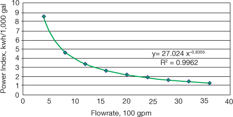
▲Figure 3. Part-load operation (i.e., operation below design capacity) reduces the efficiency and increases the energy cost of a fixed-speed centrifugal pump. It also has a hidden long-term cost — the extra cost incurred from buying oversized equipment.

Power tends to increase monotonically (quasi-linearly) with flowrate. As illustrated in Figure 3, part-load operation at fixed speed is very expensive.

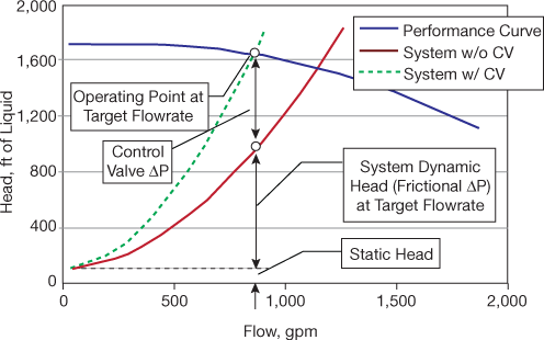
▲Figure 4. The relationship between required flow and required head is called the system curve. During throttling control, the control valve (CV) incurs a pressure loss. The system curve can be plotted without the CV pressure drop (red line). The system curve with the CV pressure drop can be plotted separately (green dashed line). The maximum flow that can be attained is at the intersection of the system curve and the performance curve when the CV pressure drop is zero.

The relationship between required flow and required head is called the system curve (Figure 4). The total pressure drop includes static head (i.e., the sum of the change in pressure plus elevation) and dynamic head (i.e., primarily frictional losses in piping, equipment, and the control valve [CV]). The control valve loss is incurred during throttling control, and is the difference between the head delivered by the pump and the head required to overcome friction in the piping and equipment. So, to calculate the minimum head (and power) that must be supplied to the fluid, first calculate static and dynamic head.

Static head (H_s) in ft of liquid is:

where P₂ is the pressure in the final destination vessel, P₁ is the pressure in the fluid supply tank, ρ is the density of the liquid, h₂ is the highest elevation to which the liquid must be pumped, and h₁ is the height of the liquid in the suction tank.

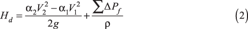
Dynamic head (H_d) in ft of liquid is:

where α₂ is the flow area of the discharge pipe, α₁ is the flow area of the suction pipe, V₂ is the velocity in the discharge pipe, V₁ is the velocity in the suction pipe, g is the gravitational constant, and ΔP_f is the frictional pressure drop in the piping system, including fittings, equipment, and instruments (1). In normal industrial piping systems, the kinetic energy component (V²/2g) is generally small and can be safely neglected.

Equations 1 and 2 are both special cases of the Bernoulli equation, which is a fundamental generalized energy balance for any fluid transport system. The frictional term in the Bernoulli equation includes pressure losses in the piping, equipment, instruments, and the pump itself (bearings, seals, etc.). It is common practice, however, to separate internal pump losses from piping/equipment losses. Internal losses within the pump are accounted for as pump efficiency, and only the piping, equipment, and instrument losses are included in the dynamic head component of the system (ΔP_f).

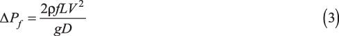
The generic equation for estimating frictional pressure drop (in consistent units) in every section of pipe with an inside diameter D and equivalent length L is:

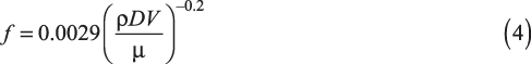
where V is the velocity in the relevant section of relevant pipe and f is the Fanning friction factor, which can be reasonably approximated for turbulent flow in standard industrial steel pipes (roughness factor ε = 0.00017 ft) as:

where μ is the viscosity. If the pipe consists of multiple sections with different diameters and lengths, you must add the individual values for ΔP_f for all of the sections.

Notice that the right-hand sides of Eq. 3 and Eq. 4 both have only one flow parameter — velocity — that varies significantly during normal plant operation. All of the other relatively constant variables can be combined into a single “constant” for the pipe as a whole:

where K_f is an empirical parameter that can be extracted from plant data and Q is flowrate.

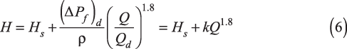
Rewriting the system curve in simplified form gives:

where H is the head in ft and the subscript d refers to an actual operating datapoint at the desired normal condition (or design specification if plant data are not available). Equation 6 is simplified by using the variable k to represent (ΔP_f)_d/(ρQ_d^1.8).

This formulation is important because it provides an easy and sufficiently accurate way to estimate the entire system curve from just four pieces of plant data — H_s, (ΔP_f)_d, Q_d, and ρ, which are usually known.

An important point to keep in mind is that the static head (H_s) seldom remains constant; in reality it fluctuates due to variations in vessel pressure at the suction and discharge ends, as well as fluctuations in liquid level in the supply or destination tanks. If frictional losses dominate the system, then for simplicity the static head may be considered approximately constant; otherwise, variations in static head must also be taken into account in the analysis.

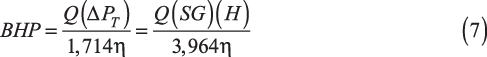
Pump power consumption (brake horsepower, or BHP) is obtained from:

where Q is the flowrate in gpm, ΔP_T is the total pressure drop including the static and dynamic head in psi, SG is specific gravity, H is head in ft liquid, and η is efficiency.

Keep in mind that the Q-H-η performance curves provided by the vendor at the time of purchase are invariably based on tests with water. If the actual fluid being pumped has a different specific gravity, the head must be adjusted by dividing H_w (the head of water, found on the performance curve) by the specific gravity of the actual fluid.

The difference between the energy supplied to the pump (the performance curve) and the pressure-volume (PV) energy absorbed by the fluid to overcome system head goes primarily into heating the fluid, with minor amounts going to valve noise and to heating the lubricating oil. For the system shown in Figure 4, the fate of energy supplied to the pump can be calculated, as in Table 1, and displayed graphically as in Figure 5.