
Sections
- Introduction to HTHA and Nelson Curves
- HTHA in liquid-filled systems
- Methods for estimating hydrogen partial pressure in liquid-filled systems
- Model components and thermodynamic models
- Example 1. Heavy cat naphtha (HCN)
- Example 2. Hydrotreater diesel
- Conclusions and recommendations
- Nomenclature
- Literature Cited
Estimate the hydrogen partial pressure of liquid-filled systems to select suitable metallurgies for industrial piping and equipment.
High-temperature hydrogen attack (HTHA) is a dangerous condition that can occur in process equipment constructed of steel and exposed to hydrogen at elevated temperatures and high hydrogen partial pressures. The Nelson Curves, maintained by The American Petroleum Institute (API) and offered through recommended practice (RP) 941, provide an authoritative guide for safe material choice to mitigate the occurrence of HTHA by relating materials selection to hydrogen partial pressure and temperature (1).
Many industries, including petrochemicals, oil and gas, biofuels, minerals, and food, are aware of the risk of HTHA caused by gas and multiphase mixtures; however, there is less experience with HTHA in liquid-filled systems. This article evaluates and recommends methods to calculate the hydrogen partial pressure of liquids so that engineers can select suitable metallurgy for liquid-filled systems.
Introduction to HTHA and Nelson Curves
HTHA is a serious problem that may occur in steel piping and equipment. Per API RP 941 (1), “… at normal atmospheric temperatures, gaseous molecular hydrogen does not readily permeate steel, even at high pressures. Carbon steel is the standard material for cylinders that are used to transport hydrogen at pressures of 2,000 psi (14 MPa).” However, at elevated temperatures, hydrogen dissociates into atomic hydrogen that is forced into the steel by high hydrogen partial pressure. The atomic hydrogen reacts with carbides in the steel to form methane gas, which accumulates in the microstructural grain boundaries. This carburization weakens the steel and, together with high methane gas pressure, increases the probability of cracking — a process known as HTHA. The empirical observation is that the risk of HTHA increases with increasing temperature and/or hydrogen partial pressure.
Nelson (2) gathered and rationalized many plant observations of HTHA on different steels. He placed boundaries on a temperature vs. hydrogen partial pressure chart to develop curves that delineate the safe operating limits for carbon and low-alloy steels (e.g., 1.25Cr-0.5Mo steels). API RP 941 (1) is the authoritative guide for safe material choice to avoid the occurrence of HTHA. It includes up-to-date results of experimental tests and actual data acquired from operating plants to establish practical operating limits for carbon and low-alloy steels in hydrogen service.
Figure 1 provides a qualitative version of a portion of Figure 1 from API RP 941 (1) to illustrate the use of Nelson Curves in materials selection for systems in high-temperature, high-pressure hydrogen service. The complete original figure includes pressures and temperatures of up to 13,000 psia (89.6 MPa) and 1,500°F (816°C). Readers should use the original figure for materials selection. For a given material, operating at conditions above its respective curve is considered unsafe, while conditions below the curve are considered safe.

▲Figure 1. This qualitative version of Figure 1 in API RP 941 describes operating limits for steels in hydrogen service to avoid high-temperature hydrogen attack (HTHA). See the original figure in Ref. 1 for details.
Materials experts typically apply a safety margin of 50°F (or a margin of 28°C) to the curves to account for uncertainties, such as process fluctuations, inaccuracies in temperature measurements, and uncertainties in calculated hydrogen partial pressures. Figure 1 indicates that carbon steel with and without post-weld heat treatment (PWHT) is vulnerable to HTHA, especially at high temperatures. Alloy steel has a higher resistance to HTHA.
For example, if the operating hydrogen partial pressure is 500 psia (3.44 MPa) and the 50°F (28°C) safety margin is applied, the following maximum operating temperatures can be obtained from Figure 1 in API RP 941 for various steels:
- carbon steel with no PWHT: 410°F (210°C)
- carbon steel with PWHT: 470°F (243°C)
- 1.25Cr-0.5Mo steel: 890°F (477°C).
The Nelson Curves are also used to select the base metal below internal stainless steel (SS) weld overlay or cladding, as hydrogen can diffuse through the SS layer and cause HTHA of the underlying base metal. The SS layer, which is typically required for corrosion resistance, can reduce the amount of hydrogen that reaches the base metal, but most materials experts do not account for this when purchasing new components.
This discussion of application of Nelson Curves from API is only for illustration purposes. Engineers who perform materials selection for process systems should consult the detailed descriptions and nuances presented in API RP 941. For certain applications, various other material degradation mechanisms must be considered in addition to HTHA, which may require SS overlay or cladding or a higher alloy than prescribed by the Nelson Curves.
HTHA in liquid-filled systems
The 8th Edition of API RP 941 (1) includes Annex G, which addresses the issue of estimating the hydrogen partial pressure in the liquid phase. Examples of liquid-filled lines containing hydrogen that have a risk of HTHA include:
- hydroprocessing unit separator liquid lines upstream of pressure letdown valves (Figure 2)
- some hydroprocessing unit feed lines and equipment where a slipstream of hydrogen is injected and then is completely absorbed by the liquid as the temperature increases (Figure 3)
- gasoline desulfurization units with pumping of the reactor bottoms streams (Figure 4)
- some biofuel units
- certain coal liquefaction units
- certain gasification units.
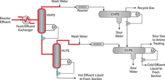
▲Figure 2. A four-drum hydroprocessing unit includes hot and cold high-pressure separators (HHPS and CHPS) and hot and cold low-pressure separators (HLPS and CLPS). Liquid-filled operating lines to be evaluated for HTHA risk are shown in blue, and gas-containing lines and vessels to be evaluated for HTHA risk are shown in red.
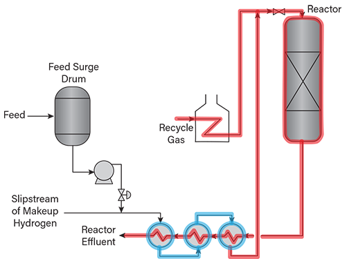
▲Figure 3. This hydroprocessing unit has a gas-only heater and a slipstream of hydrogen (i.e., soak gas) injected into the liquid feed. Soak gas may fully dissolve in the feed, especially upon heating. Liquid-filled operating lines to be evaluated for HTHA risk are shown in blue, and gas-containing lines and vessels to be evaluated for HTHA risk are shown in red.

▲Figure 4. This gasoline desulfurization column with hydrogen injection upstream of the reboiler may be at risk for HTHA. Liquid-filled operating lines to be evaluated for HTHA risk are shown in blue, and gas-containing lines and vessels to be evaluated for HTHA risk are shown in red.
Figures 2, 3, and 4 depict sections of various hydro-processing units at risk of HTHA. Vapor-only and mixed-phase sections, for which hydrogen partial pressures can be easily estimated, are shown in red, and liquid-filled sections are shown in blue.
The goal of this article is to evaluate and improve estimates of the partial pressure of hydrogen in the liquid phase so that the Nelson Curves in API RP 941 may be used to identify materials of construction that will be safe for the intended operating conditions.
Instead of hydrogen partial pressure, Cheluget (3) correctly identified hydrogen fugacity as the thermodynamic driving force for HTHA. This article focuses on hydrogen partial pressure due to its legacy of use in the evolution of the Nelson Curves. However, some of the methods to determine hydrogen partial pressure proposed in this article use the hydrogen fugacity.
This article presents five methods to estimate the hydrogen partial pressures of liquids and analyzes the validity and accuracy of each method. Design engineers can use this information to choose the most appropriate method to estimate the hydrogen partial pressure of their particular liquid-filled system. The choice of method also depends on the options available within the simulation software, for example, whether it reports fugacity coefficients.
Methods for estimating hydrogen partial pressure in liquid-filled systems
The five methods to estimate hydrogen partial pressure in liquid are explained using the process-simulation flowsheet presented in Figure 5. The stream FEED in this simulation model is two-phase at temperature TA and pressure PA, and the vapor hydrogen mole fraction is equal to yH2,A. The hydrogen partial pressure of the liquid at Condition A is the product of the pressure PA and the vapor hydrogen mole fraction yH2,A.
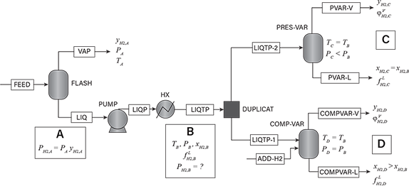
▲Figure 5. A simulation flowsheet can be used to explain the five methods to calculate hydrogen partial pressure in liquids.
The liquid at Condition A may be subject to a variety of temperature and pressure changes. In the flowsheet depicted in Figure 5, it is pumped to a higher pressure PB, and a combination of pumping and heat exchange changes the liquid temperature to TB. At temperatures above 400°F (204°C), hydrogen solubility usually increases with temperature. Hence, increasing the temperature at fixed pressure and liquid concentration tends to lower the hydrogen partial pressure. Regardless of the processing steps, the goal is to estimate the hydrogen partial pressure at Condition B, and it is not recommended to use any upstream values of the hydrogen partial pressure that may be available (e.g., Condition A).
We need to estimate the hydrogen partial pressure of the liquid at Condition B. The temperature, pressure, and composition of the liquid are known, but the liquid does not have a vapor phase in equilibrium with it. The recommended approach is to artificially create an incipient vapor phase, and then relate the partial pressure at Condition B to the hydrogen partial pressure of the stream for which the vapor phase has been created. The proposed calculational procedure duplicates the stream at Condition B into two identical streams. The first duplicated stream enters block PRES-VAR where its pressure is reduced isothermally such that the stream moves to its bubble point (Condition C) — i.e., a vapor phase is formed by pressure reduction at temperature TB. The vapor phase formed at Condition C has a hydrogen mole fraction yH2,C, and this mole fraction would be equal to yH2,A if TB equaled TA.
The second stream enters block COMP-VAR, where a vapor phase is created by adding pure hydrogen such that the mixture is moved to its bubble point at pressure PB and temperature TB (Condition D). In doing so, the liquid mole fraction of hydrogen increases from xH2,B to xH2,D, and a vapor phase with hydrogen mole fraction yH2,D is formed.
The following sections describe the five methods to estimate the hydrogen partial pressure.
I. Pressure variation: Low. The hydrogen partial pressure is assumed to be the partial pressure of the vapor phase at Condition C, i.e., when the pressure is lowered to its bubble pressure, PC.

where PH2,I is the calculated hydrogen partial pressure at Condition B and yH2,C is the hydrogen vapor mole fraction at Condition C.
PH2,I depends on the temperature and composition at Condition B, but is independent of pressure PB. This method is not recommended because it ignores the Poynting effect, which must be considered when increasing the pressure from PC to PB (for an example, see Ref. 4). API RP 941 calls this the conventional thermodynamics method, and it is retained for historical purposes.
II. Pressure variation: High. The pressure variation: high method is similar to Method I, but it assumes hydrogen partial pressure is the product of the vapor mole fraction at Condition C and the pressure PB (rather than PC).

This method too has no basis in thermodynamics, but has been retained for historical purposes. API RP 941 calls this approach the total pressure method.
III. Fugacity equivalency method. In the fugacity equivalency method, the liquid fugacity of hydrogen at Condition B, f LH2,B, is calculated by the thermodynamic model. The hydrogen partial pressure can be calculated by dividing the liquid fugacity by the fugacity coefficient. The hydrogen fugacity coefficient of the vapor at Condition D, φVH2,D, can be used because the temperature and pressure are the same as those of Condition B, and the fugacity coefficient is assumed to be a weak function of hydrogen mole fraction in the vapor phase.

IV. Fugacity correction method. In the fugacity correction method, the ratio of the hydrogen partial pressures at Conditions B and C is assumed to be equal to the ratio of the hydrogen liquid fugacities at Conditions B and C.

The correction factor in this method is equivalent to the Poynting correction presented in most textbooks on thermodynamics (for an example, see Ref. 4). Here, the ratio of liquid fugacities accounts for the effect of increasing the pressure from PC to PB.
V. Composition variation and compensation method. In the composition variation and compensation method, the ratio of the hydrogen partial pressures at Conditions B and D is assumed to be equal to the ratio of the hydrogen liquid mole fractions at Conditions B and D.

where xH2,B and xH2,D are the hydrogen liquid mole fractions at Conditions B and D, respectively.
Method V is similar to Method III. The use of the ratio of mole fractions in Method V offers a way to estimate the hydrogen partial pressure without having to calculate fugacities, as this reporting capability may not be available in some commercial software products.
Summary of methods. The five methods to estimate the hydrogen partial pressure of a liquid stream may be summarized and compared as follows:
- All five methods have the same limiting value of hydrogen partial pressure when PB approaches PC, i.e., when Condition B is at the bubble point. Hence, there is at least some measure of consistency among all five methods, and similarities with the usual calculation of hydrogen partial pressure for systems that contain a vapor phase.
- Method III has the strongest basis in thermodynamics, and therefore the other four methods are evaluated relative to Method III.
- Methods I and II are not justified by thermodynamics for conditions downstream of pumps or heat exchangers, but are retained for historical purposes.
- Methods I, II, and V do not require fugacities or fugacity coefficients, as these thermodynamic properties may not be available in certain process-simulation software packages.
Model components and thermodynamic models
The following two examples assess the accuracy of the five methods. Example 1 illustrates how the calculated hydrogen partial pressure decreases with increasing temperature as the hydrogen solubility increases. Example 2 shows how the calculated hydrogen partial pressure depends on the chosen thermodynamic model and the correlation parameters of the model.
To clearly demonstrate the various effects and enable reproducible calculations, the examples use known compounds (rather than pseudocomponents) to represent the chemical components in the systems, as well as common and widely accepted thermodynamic models. Table 1 presents the chemical compounds used in the examples and the model parameters.
| Table 1. The following components and properties are used in the example calculations. | ||||
| Component | Critical Temperature, °F | Critical Pressure, psia | Acentric Factor (ω) | H2 SRK kij with Solvent |
| Hydrogen | –399.9 | 190.4 | –0.216 | – |
| n-Undecane | 690.5 | 282.8 | 0.530 | 0.064 |
| n-Dodecane | 724.7 | 264.0 | 0.576 | 0.081 |
| n-Tetradecane | 755.3 | 243.7 | 0.617 | 0.101 |
| n-Hexadecane | 841.7 | 203.1 | 0.717 | 0.185 |
Both analyses use the Soave-Redlich-Kwong (SRK) equation of state (5), and a simple model that assumes an ideal liquid with a Poynting correction and determines hydrogen solubility using Henry’s law (for details, see Ref. 4).
Example 1. Heavy cat naphtha (HCN)
The sketch shown in Figure 6 presents typical processing conditions for a heavy cat naphtha (HCN) process. A narrow-boiling-range HCN is drawn from a high-pressure separator operating at 650°F and 310 psia, in which the hydrogen partial pressure is 124 psia. The hydrocarbon liquid has a boiling range of 384–443°F, and is assumed to be composed of n-undecane, n-dodecane, and n-tridecane with mole percentages of 33.9, 15.5, and 50.6, respectively.
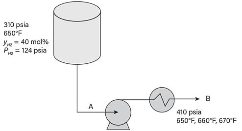
▲Figure 6. This sketch indicates the conditions of the heavy cat naphtha (HCN) vapor-liquid separator, pump, and heat exchanger described in Example 1.
The pump increases the pressure by 100 psi, and the heat exchanger increases the temperature from 650°F to 670°F in increments of 10°F. Figure 7 provides a graphical representation of the pressure and hydrogen composition variations needed to move the system from Condition B to the bubble points corresponding to Condition C and Condition D in Figure 5. Table 2 presents the hydrogen partial pressures calculated by the five methods.

▲Figure 7. Bubble pressure of the system in Example 1 at 650°F is plotted as a function of hydrogen liquid mole fraction (solid line). A vapor phase can be made to appear from the liquid of interest (Point B) by decreasing the pressure at the base hydrogen mole fraction (Point C), or increasing the hydrogen mole fraction at the base pressure (Point D).
| Table 2. Hydrogen partial pressure was calculated for the liquid from the HCN separator in Example 1 by the five methods using the SRK equation of state at 410 psia and various temperatures. | |||||
| Temperature, °F | H2 Partial Pressure, psia | ||||
| Method I Pressure Variation: Low | Method II Pressure Variation: High | Method III Fugacity Equivalency | Method IV Fugacity Correction | Method V Composition Variation and Compensation | |
| 650 | 124 | 164 | 145 | 138 | 135 |
| 660 | 111 | 146 | 133 | 125 | 122 |
| 670 | 99 | 129 | 120 | 112 | 110 |
Analysis of the results in Table 2 reveals:
- Relative to Method III, the estimations from Methods I, IV, and V are low, while the results from Method II are high.
- Methods IV and V agree with Method III to within 10%.
- If the software used has the capability to report fugacities and fugacity coefficients, Method III is recommended. If not, Method V is an acceptable alternative.
Table 2 also shows how the hydrogen partial pressure changes as the temperature increases. Since the solubility of hydrogen increases as the temperature increases, the calculated hydrogen partial pressure decreases with increasing temperature.
Based on the Nelson Curves in API RP 941 and the hydrogen partial pressure and temperature in the liquid-filled lines, a minimum of 1.0Cr-0.5Mo material is needed to resist HTHA. Higher alloys (e.g., Type 321 SS) may be needed if there are also other concerns such as sulfidation — i.e., corrosion caused by sulfur compounds at high temperature.
In the past, some designers mistakenly assumed that there was no hydrogen in liquid-filled lines, or that the hydrogen partial pressure was the value estimated by Method I. This has led to leaks in carbon steel piping and the need for material upgrades after the problem was discovered.
Example 2. Hydrotreater diesel
The system presented in Figure 8 simulates the liquid line from a hydrotreater vapor-liquid separator. The vapor from the separator has a hydrogen concentration of about 97 mol%, which corresponds to a hydrogen partial pressure of 634 psia. We wish to estimate the hydrogen partial pressure of the liquid that has been pumped to 800 psia while maintaining the temperature at 550°F. The mixture is modeled as a hydrogen and n-hexadecane binary mixture; n-hexadecane (i.e., cetane) is a good approximation for diesel fuel.

▲Figure 8. The liquid line exiting a hydrotreater vapor-liquid separator and pump may be vulnerable to high-temperature hydrogen attack (HTHA).
The hydrogen partial pressures, estimated at the pump discharge, are presented in Table 3 (using the simple model with Henry’s constant) and Table 4 (using the SRK equation of state). Figure 9 shows how the estimated hydrogen partial pressures from the five methods compare, and using the SRK equation of state, how they change as the pressure is increased from PA and the temperature is maintained at 550°F.
| Table 3. Effective hydrogen partial pressures were calculated in Example 2 with the five estimation methods using a simple model with Henry’s constant for the thermodynamic correlations. | |||||
| Method I Pressure Variation: Low | Method II Pressure Variation: High | Method III Fugacity Equivalency | Method IV Fugacity Correction | Method V Composition Variation and Compensation | |
| H2 Partial Pressure | 633.7 | 779.9 | 646.4 | 648.7 | 646.4 |
| %Difference | –2.0 | 20.7 | 0 | 0.3 | 0.0 |
| Table 4. Effective hydrogen partial pressures were calculated in Example 2 with the five estimation methods using the Soave-Redlich-Kwong (SRK) equation of state. | |||||
| Method I Pressure Variation: Low | Method II Pressure Variation: High | Method III Fugacity Equivalency | Method IV Fugacity Correction | Method V Composition Variation and Compensation | |
| H2 Partial Pressure | 633.4 | 779.6 | 661.2 | 663.1 | 650.7 |
| %Difference | –4.2 | 17.9 | 0 | 0.3 | –1.6 |
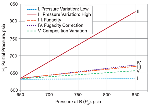
▲Figure 9. This graph shows variation in the calculated hydrogen partial pressure as a function of PB using the SRK equation of state (Table 4) as the temperature is maintained at 550°F and the pressure is varied from 650 psia to 850 psia.
In this example, the hydrogen partial pressure and temperature in the liquid-filled lines again shows that a minimum of 1.0Cr-0.5Mo material is needed to resist HTHA. Higher alloys may be needed if there are other concerns, such as sulfidation, in addition to the risk of HTHA.
The chosen thermodynamic model causes only minor differences in this example. The calculated hydrogen partial pressure using Method III and the SRK model (5) (661 psia, Table 4) is higher than that calculated by the simple model with Henry’s constant (646 psia, Table 3), but only by 2%. This small difference is likely within the experimental uncertainty. The differences are small because the two methods have been correlated using the same vapor-liquid equilibrium data; larger differences may result when the phase equilibrium predictions from the models are based on different experimental data or come from generalized correlations.
Conclusions and recommendations
When determining the hydrogen partial pressure in liquid-filled lines, Methods I and II are not justified by thermodynamics. They have only been included in this article for historical purposes, and their use should be avoided in favor of Methods III, IV, or V, which all provide similar results. Method III is the preferred option if fugacities are reported by the software used. If fugacities are not reported by the process-simulation software, Method V is an acceptable alternative. It is recommended to validate the accuracy of the thermodynamic models using experimental data for the relevant phase equilibrium.
The methods and analyses presented in this article enable engineers to accurately estimate the hydrogen partial pressure of liquid mixtures. These estimates can then be used by process design and operations engineers, in collaboration with materials engineers, to select suitable metallurgy to mitigate HTHA.
Literature Cited
- American Petroleum Institute, “API Recommended Practice 941, Steels for Hydrogen Service at Elevated Temperatures and Pressures in Petroleum Refineries and Petrochemical Plants,” 8th ed., www.api.org/products-and-services/standards (Feb. 2016).
- Nelson, G. A., “Hydrogenation Plant Steels,” 1949 Proceedings, Vol. 29M, API, Washington, DC, pp. 163–174 (1949).
- Cheluget, E., “Prediction of the Fugacity of Hydrogen Gas Dissolved in Organic Solvents with Emphasis on the High-Temperature High-Pressure Subcooled Liquid State,” presented at the 2019 AIChE Annual Meeting, Orlando, FL, (Nov. 10–15, 2019).
- Poling, B. E., et al., “The Properties of Gases and Liquids,” 5th ed., McGraw-Hill, New York, NY (2001).
- Soave, G., “Equilibrium Constants from a Modified Redlich-Kwong Equation of State,” Chemical Engineering Science, 27 (6), pp. 1197–1203 (June 1972).

Copyright Permissions
Would you like to reuse content from CEP Magazine? It’s easy to request permission to reuse content. Simply click here to connect instantly to licensing services, where you can choose from a list of options regarding how you would like to reuse the desired content and complete the transaction.