Troubleshooting Process Control Problems

Identifiying and troubleshooting problematic control loops can significantly improve plant performance.

The theoretically attainable performance of a plant in the chemical process industries (CPI) is closely aligned with the technology applied and the equipment installed during its design and construction. Achieving that potential performance depends on proper equipment operation, which depends in part on the effectiveness of the plant’s control system. For decades, the CPI have tried to close the gap between actual and potential plant performance through the application of advanced control.

Numerous opportunities exist to improve plant operation through the rectification of the basic regulatory control system without the application of advanced control. In fact, some of the benefit that is attributed to advanced control technology is often the result of correcting regulatory control problems during the implementation of an advanced control project.

Systematic methods can be used to identify problematic regulatory control loops. Once identified, straightforward techniques are available to troubleshoot several typical control system problems. This article describes these methods and techniques.

Identifying problematic control loops

While some control loop problems may be well known to plant personnel, others may be more obscure. Therefore, the first step of correcting a regulatory process control system is identifying the problematic loops.

Begin by identifying loops that are continuously operated in manual mode. Operators quickly lose patience with controllers that do not work well, so this is a key indicator of a problem. In some cases, primary controllers can remain in automatic mode even though they have tracking or conditional status because the downstream secondary controller or function block is not in the preferred mode or position. Therefore, it is also necessary to look at the status of the controller to confirm whether it is in use.

Next, ask the following questions to help identify regulatory control loops with low service factors or problematic performance:

• Do any controllers typically exhibit a large degree of variability or oscillatory/cyclic behavior?
• Are any control loops periodically placed in manual mode to handle large disturbances, implement setpoint changes, or squelch unstable control responses? This is common, for example, during cracking heater swaps and dryer switches in ethylene plants.
• Do any controllers typically require a very long time to reach their setpoint following a disturbance, process excursion, or setpoint change?
• Do operators frequently change the setpoint of some controllers?

Those questions can be answered easily by applying common statistical functions to data extracted from the plant’s data historian or distributed control system (DCS). One simple approach is to import time series data (e.g., one-minute data for a week) for the relevant control parameters of all the plant control loops into a spreadsheet where the analysis can be performed. While some effort is required to prepare the spreadsheets, they can be used repeatedly on a periodic basis to quickly identify new or developing problems.

• Service factor. Convert the mode and status states to a numerical value (e.g., IF mode = manual or status = conditional/tracking, THEN value = 0, ELSE value = 1) for each data point in the time series. The average value across the entire time series represents the service factor for the controller (Figure 1). Service factors between 0% and 50% are poor. Service factors between 50% and 90% are non-optimal, and the controller may be adversely affected by particular disturbances. Service factors greater than 90% are good.
• Controller performance. Multiple calculations are required to analyze controller performance. First, calculate the difference between the setpoint and the process variable of the controller for each available data point (the result can be positive or negative). Then, calculate the standard deviation for the full array of those calculated difference values. The standard deviation value divided by the range of the controller (e.g., if the range is –50°F to 50°F, the range is 100°F) provides an excellent normalized indication of the controller performance (Figure 2). Focus on the controllers with the highest values to identify the controllers with the most significant performance issues. In the statistical analysis example in Figure 2, Tag #2 should be addressed first.
• Setpoint variance. Operators sometimes try to help a level, pressure, or temperature controller respond to a disturbance by changing its setpoint to accelerate the control response, instead of allowing the controller to do its job. A high normalized variance (i.e., variance divided by the range of the controller) of the setpoint over the duration of the time series indicates such a controller.

---

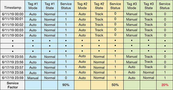
▲Figure 1. Statistical analysis can help identify problematic control loops. In this example, the service factor is calculated to determine which controller should be prioritized for troubleshooting. Tag #3 should be prioritized because it is only in service 20% of the time (assuming it is not a situational controller that is used only during limited types of operation).

---

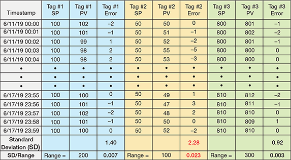
▲Figure 2. The normalized standard deviation is another statistical analysis tool for evaluating controller performance. In this example, Tag #2 has the highest normalized standard deviation and thus should be prioritized for troubleshooting first.

Statistics may not capture all of the issues, so conducting discussions with several plant operators may identify additional problematic control loops. When doing so, it is best to talk with operators from several different shifts because different shifts can have different approaches to the same operating and control issues.

Once you have compiled a shortlist of underperforming control loops, troubleshooting can begin. The two troubleshooting techniques addressed in this article are systematic review of general control loop functionality and examination of specific control loop structures.

Troubleshooting general control loop functionality

Many problems can be eliminated by methodically reviewing the general functionality of the problematic control loops.

Tuning. Controller tuning is frequently blamed for regulatory process control problems, although it is often not the culprit. Tuning procedures will not be addressed in this article because they are widely covered in the literature.

Because control systems from different vendors use different control equations, be cognizant of whether the control equations use proportional band or gain, interactive or independent gain, resets per minute (or second), or integral time per reset when selecting your tuning constants. In addition, if a controller appears to work well in some scenarios and not well in others, consider whether adaptive tuning is required.

A good example of an application requiring adaptive tuning is the coil outlet temperature (COT) controller on an ethylene plant’s cracking heater. The COT controller is typically tuned during normal cracking operation, when an endothermic cracking reaction is absorbing much of the fired duty. However, during decoking operations, an exothermic combustion reaction occurs in the radiant coils. Therefore, the response of the COT controller to a step change in the fuel firing is quite different in those two operating modes. Adaptive tuning can be used to automatically modify the gain of the COT controller during decoking operations to account for this change in response.

Other cases in which adaptive tuning might be applicable include:

• split-range controllers
• cascade loops with multiple secondary controllers
• controllers in nonlinear processes in which the process gain changes significantly as the plant load changes (i.e., 100% capacity operation vs. turndown at 70%, etc.)
• controllers that can normally operate across their entire control valve range.

Instrument reliability, range, and calibration. For controllers that operate mainly in manual mode (or tracking/conditional status), check whether the measured process variable is reliable. Trend the measured process variable while the controller is in manual mode and the associated control valve is at a constant opening. Look for the following characteristics as an indication of an instrumentation problem:

• the value is constantly frozen at the low or high end-of-scale value (the instrument might not be scaled properly or might be installed incorrectly)
• the value exhibits high-frequency noise with a large amplitude
• the value appears to be relatively constant and then exhibits large jumps in value.

These measurement behaviors may be due to instrumentation problems, such as:

• installation mistakes (inversion of a flow orifice, insufficient space between flow element and control valve, etc.)
• mismatch between the installed thermocouple type and the defined transmitter type
• incorrect calibration, such as calibrating a level measurement for a density that does not match that of the liquid in the vessel (this can produce a significant error in the form of blow-through [i.e., the actual level is lower than the reading] or carryover [the actual level is higher than the reading]).

Troubleshoot the instrumentation’s installation before moving on to the control loop configuration.

---

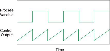
▲Figure 3. Valve stiction occurs when the valve does not move after a change request is sent to its actuator from the controller. As a consequence, the controller’s output signal continues to change until the actuator generates enough force to move the valve. When the valve finally moves, it creates a large step change in the measured process variable.

Final control elements. If a controller exhibits oscillatory or highly variable performance when in automatic mode, check the control valve and its associated hardware. In particular, if the controller output appears as a sawtooth pattern and the process variable exhibits a square-wave response (as in Figure 3), then valve stiction could be the problem.

To quickly test for valve stiction, place the controller in manual mode and maintain a constant valve opening. If the measured variable stabilizes, then control valve stiction could be the source of the problem. The valve could be sticking because the packing is too tight or because there is friction between the valve seat and disc combined with an underpowered actuator. Alternatively, the final control element (i.e., actuator, positioner, etc.) could have a deadband that does not initiate a valve movement until a threshold value is reached. This can be easily adjusted, but is occasionally set too wide by well-intentioned instrument engineers who are trying to extend the valve life by minimizing thrashing of the valve.

A stroke test is often used when troubleshooting this issue. However, large changes in output during a stroke test usually apply enough force to move even the stickiest valve, which will mask the problem. Small incremental changes in output should be used in such cases.

Mismatch between the controller output signal and the actual valve position can result in a loss of control range for the valve. If the problem continues to reoccur after recalibration, then installation of a smart positioner might be warranted.

---

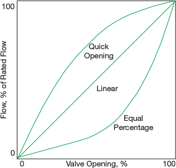
▲Figure 4. The control valve characteristic curves are generated by plotting the flow (percent of rated flow) against valve opening. Each control valve requires the correct trim to produce the appropriate response for a particular process control application.

In addition, each valve has a particular type of trim that provides for more reliable response (i.e., linear) in a particular region of the valve opening (Figure 4). If the valve has the wrong trim for the application or if the process can operate in multiple regions of the valve opening, then the valve may not be operating in its optimal region and the controller performance can degrade. If the trim cannot be changed, adaptive tuning may solve the problem.

Control equation. Within a vendor’s control system, it may be possible to select one of several control equations. Although these equations have the same structure, they contain subtle differences that affect the control loop response. Depending on the equation selected for a particular application, each of the control terms — i.e., the proportional (Kp), integral (Ki), and derivative (Kd) terms — can act on either a function of the controller error (i.e., setpoint minus the measured value) or a function of the process variable.

In most situations, the proportional and integral terms should act on the error and the derivative term should act on the process variable for two reasons. First, if the proportional term acts on the process variable instead of the error, then there will not be a proportional kick whenever the operator changes the setpoint. This can produce a very sluggish response to setpoint changes, which some operators interpret as a reason to maintain the controller in manual mode. Second, if the derivative term acts on the error, then the derivative action (which responds to rate of change) can overreact to setpoint changes and cause a rapid rate of change in the error.

With new smart devices that perform control logic in the field rather than in a common location (e.g., the DCS), a variety of possible control equation structures may be employed at a single plant site due to the different smart device vendors using different control equations. It is therefore important to confirm which control equations are used in which devices.

Control action and valve failure mode. If a controller is always in manual mode or is unstable when it is not in manual mode, check that the control action is configured properly. Controllers are either specified as direct or reverse, which defines whether the controller output increases (direct) or decreases (reverse) when the measured process variable increases. If the controller is designated with the wrong control action, it will become unstable almost immediately upon activation — within minutes in most cases.

---

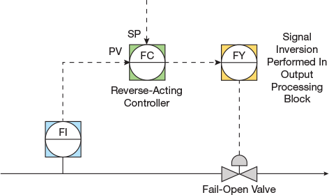
▲Figure 5. A signal output inversion is usually invisible to the operator. Here, it is configured in an output processing block in the control system.

Also check the valve failure mode in combination with the control output processing. Output signals from the control system to the valves in the field are normally displayed such that 100% represents a fully open valve and 0% represents a fully closed valve. For valves that use a signal to close (i.e., fail-open valves), the inversion of the controller output is usually performed in a manner that is invisible to the operator. The inversion commonly takes place in the positioner or is accomplished by configuration of an output processing block in the control system (Figure 5). If this inversion is not implemented properly, the effect on control performance is the same as if the control action was configured incorrectly — i.e., the control response will be unstable.

Setpoint tracking and initialization. If a controller exhibits a significant disturbance when it is initially placed in service but eventually stabilizes, then it is possible that the controller’s setpoint tracking and/or initialization was not configured properly.

---

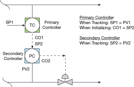
▲Figure 6. A cascade control scheme performs slightly differently during initialization than during standard operation. During initialization, the output of the primary controller tracks the setpoint of the secondary controller (i.e., CO1 is set equal to SP2). However, when the secondary controller is in manual mode (i.e., tracking), its setpoint tracks its process variable (i.e., SP2 is set equal to PV2).

Initialization is primarily an issue with cascade and other multilevel control strategies. In these cases, the output of the primary (i.e., higher-level) controller is set equal to the equivalent value of the setpoint of the secondary (i.e., lower-level) controller when the secondary controller is not in the mode that allows it to receive a setpoint (Figure 6). Most control systems automatically provide this type of initialization when control functions are connected to each other, although there are some special cases in which this does not happen.

The more common problem is improper setpoint tracking. Setpoint tracking refers to whether or not the value of the controller’s setpoint is automatically adjusted to equal the value of the process variable when the control algorithm is not in service (i.e., manual mode or tracking status). If setpoint tracking is configured, then the initial error (i.e., setpoint minus process variable) will be zero when the controller initializes and the controller output will initialize smoothly (i.e., the control output will not bump when the control algorithm first executes). Most controllers are configured for setpoint tracking, but there are some special cases in which setpoint tracking should not be used, such as:

• override controllers (e.g., a high-level override that prevents carryover of liquid into a vapor stream)
• relief controllers (e.g., a high-pressure relief controller on a tower that sends the overhead stream to a flare if the pressure is too high)
• equipment protection controllers (e.g., a minimum-flow protection controller on a pump).

In each of these three cases, the correct setpoint for the controller is based on the safety of the equipment, which in turn depends on its design. Therefore, once determined, the setpoint should never change in those special cases. If setpoint tracking is used on these types of controllers, then the setpoint will reset to the current process variable value when the controller is placed in manual mode. For example, if an override controller is placed back in service with its setpoint equal to the process variable value, then the controller will immediately override its primary controller and perform poorly.

---

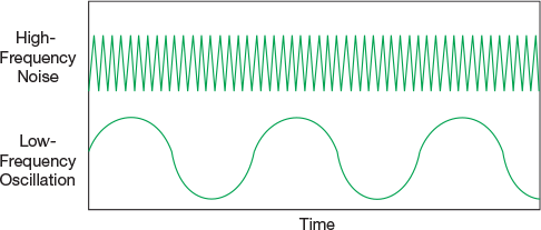
▲Figure 7. A process variable exhibiting high-frequency signal noise can produce unstable control by causing the proportional action to overreact and make large changes.

Input filtering and variable clamping. If a controlled variable is highly oscillatory or extremely sluggish, it could be due to improper input filtering. A process variable exhibiting high-frequency signal noise (Figure 7) can produce unstable control by causing the proportional action of the associated controller to overreact and rapidly make large changes to the controller output. Filtering can improve this situation, but it should only be used to alleviate high-frequency noise. Use of filtering to attenuate low-frequency oscillation will elongate the oscillation and make it more difficult to control.

On the other hand, if the control response is sluggish, watch out for double dipping on the filtering. Some transmitters have filtering applied in the field. If the signal is filtered again in the DCS or programmable logic controller (PLC), the signal may be made too sluggish. A first-order filtering constant of 1–5 sec is normally sufficient to squelch high-frequency noise, regardless of where it is employed.

Troubleshooting specific control loop structures

While problems can occur in any loop, control loops with certain features are more prone to non-optimal implementation that can lead to poor performance. When you are trying to identify problematic loops, pay special attention to:

• primary controllers with multiple cascaded secondary controllers
• control loops with overrides
• split-range controllers
• level controllers with gap action
• controllers that use calculated input values
• controllers that use inputs from gas chromatography (GC) analyzers.

If a problematic loop falls into one of these special categories, you should check the controller for common configuration errors.

Primary controllers with multiple cascaded secondary controllers. A standard cascade control loop has one primary controller and one secondary controller, and the output of the primary controller sets the setpoint of the secondary controller (Figure 6).

---

▲Figure 8. A single tower pressure controller adjusting flow to multiple condensers, an example of a primary controller with multiple secondary controllers, has a nonstandard initialization mechanism and requires customization.

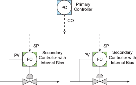
However, when a cascade structure has one primary controller and multiple secondary controllers, such as a tower pressure controller adjusting flow to multiple condensers (Figure 8), the initialization mechanism is nonstandard and requires customization. So, it is more likely to be implemented incorrectly. If the two secondary controllers are operating in automatic mode with two different setpoints, then the output of the primary controller cannot initialize to both of the secondary controller setpoints simultaneously (since it can only be set to a single value). In this case, when it initializes, it will send the same output to both secondary controllers, which will change one of the setpoint values (assuming they did not both start with the same value); this is often referred to as bumping.

If such a cascade structure exhibits an initialization problem, the problem can be overcome with the use of internal biases in the secondary controllers. The internal biases would be applied to the setpoints of each secondary controller to compensate for the difference between the primary controller output value and the individual secondary controller setpoint value.

Note also that the gain of the primary controller will change, depending on how many secondary controllers are in service. In the example shown in Figure 8, when the primary pressure controller output signal changes by 1%, flow to the condensers will change by 1% when both of the condenser flow controllers are in service (i.e., both secondary flow controllers are in cascade mode). However, it will change by only 0.5% if one of the two condenser controllers is not in cascade with the primary pressure controller. Therefore, the gain of the control response is significantly different depending on how many of the secondary flow controllers are in cascade mode. This can be addressed by applying adaptive tuning logic (also called gain scheduling) to the primary pressure controller based on the number of secondary flow controllers that are in cascade mode.

---

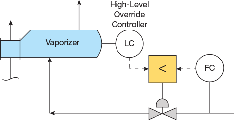
▲Figure 9. In this example of an override control strategy, the process liquid into the vaporizer is controlled at a specific flowrate unless the liquid level in the vaporizer reaches its high-level override setpoint. If that occurs, the control output signal from the high-level override controller will become less than the control output signal from the flow controller, which will cause the valve opening to be reduced (thereby reducing the flow) and prevent the level from rising higher.

Control loops with overrides. A simple override control loop has one primary controller and one override controller, plus a signal selector that selects the higher or lower of the two controller output signals, depending on the objective of the override (Figure 9). An override controller normally operates with an offset between its setpoint and measured variable. Therefore, unless the system is configured with external feedback from the selector output to each of the controllers in the override loop, the nonselected controller typically continues to change its output (i.e., called windup) and reaches its minimum or maximum output value (Figure 10). Some DCS and PLC systems automatically incorporate this logic when an override control function is configured, whereas others require the configuration engineer to specify it. In the latter case, when it is not done properly, the ensuing performance issue often motivates operators to place the override controller in manual mode and set its output to either 0% or 100% to avoid any interference with the primary loop. This essentially negates the existence of the override.

---

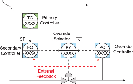
▲Figure 10. The controllers in an override strategy must be configured with external feedback to update the value of the nonselected control output so that it does not wind up (i.e., continue to change its output).

Split-range controllers. A split-range controller sequentially adjusts more than one downstream controller or valve in series based on the value of its control output signal. For example, as shown in Figure 11, the output of a split-range temperature controller can be sent to two control valves. As the temperature increases, Valve A is closed from 100% open to 0% open as the controller output value changes from 0% to 50%. Then, Valve B opens from 0% open to 100% open as the controller output value changes from 50% to 100%.

---

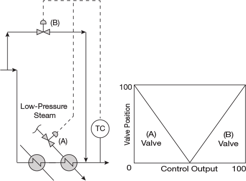
▲Figure 11. A split-range controller adjusts more than one controller or valve in series. Here, the temperature controller closes the steam valve (A) first and then opens the bypass valve (B) to reduce the temperature.

Split-range controllers are notorious for working well some of the time, but not always. There are several potential causes (and remedies) for this issue.

If the process response of the two valves is different — i.e., changing one of the valves by 1% changes the value or dynamics of the process variable differently than a 1% change in the other valve — then a single set of tuning constants may not be optimal for performance across the entire range of operation. In this case, adaptive tuning, gain, or scheduling may be required.

If the installed valves have very little sensitivity at the ends of their valve opening range — i.e., if there is very little change in flow between a valve opening of 0% to 5% or 95% to 100% — then there will be a deadband in the response of the split-range controller in the transition region between the two valves. In this case, it may be necessary to overlap the action of the two valves (i.e., start opening Valve B at a controller output value of 45% and do not fully close Valve A until the controller output value reaches 55%).

Level controllers with gap action. A gap-action level controller responds differently when the difference between the setpoint and process variable (referred to as controller error) is less than the specified gap than when the difference is greater than the specified gap. A gap-action controller is often used to allow the level in a vessel to float between high and low limits (i.e., a gap) without taking any control action to change the flow to the downstream equipment.

---

▲Figure 12. This example shows the integrating effect of a simple level control response. Unlike typical process control responses, levels do not achieve a new steady-state value when a disturbance is imposed. If the liquid feed rate (i.e., FC1) to the vessel increases while the liquid outlet flow (i.e., FC2) remains constant, then the liquid level (i.e., LC) will continue to increase until the liquid overflows the vessel.

This type of strategy is often applied in a manner that increases instability in the system. Applying gap-action level control with a zero gain inside the gap subjects the process to an integrating effect. For example, a step change in the feed flowrate to the vessel will eventually overflow or empty the vessel if no adjustment is made to the outlet flow (Figure 12). As a result, the level may bounce between the gap limits and create large changes in the flow to the downstream equipment when crossing the gap limits. Using a smaller, nonzero gain inside the gap may minimize the effect on downstream equipment and eliminate the continuous oscillation caused by frequently bouncing between the two gap limits. A larger gain would be used outside of the gap limits to handle severe disturbances that occur much less frequently.

Controllers that use calculated process variables. The power of the DCS has encouraged the implementation of many loops that use a calculated value as their process variable. The basic calculation and control is normally quite straightforward, but these loops are vulnerable to a few hidden pitfalls.

---

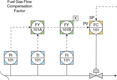
▲Figure 13. This controller uses calculated process variables. The fuel gas flow is compensated for temperature and pressure. When the noncritical variable (temperature or pressure) is out of range, the flow calculation may be inaccurate.

Consider the simple example of a flow controller that is compensated for temperature and pressure shown in Figure 13. The pitfall occurs when the quality of the noncritical variable (i.e., temperature or pressure) signal drifts out of its normal range or changes to a bad status due to instrumentation error. Depending on how the configuration was designed, one of several things could happen:

• the calculated flow reading is inaccurate
• the calculated flow value experiences a bump that causes the controller to respond erroneously
• the controller is automatically changed to manual mode operation.

These problems can be mitigated by applying the following logic:

• clamp the noncritical inputs within reasonable bounds to protect against signal drift
• install logic to continue to use the last good value of a noncritical input if its status becomes bad (which allows the controller to continue to operate based on the value of the critical input).

A heat duty controller is another example of a controller with a calculated input.

Controllers with measured process variables from GC analyzers. The input from a GC analyzer requires special processing; such processing steps may have been neglected during controller implementation. A GC analyzer sends a new analysis value on an intermittent basis (e.g., once every 3–5 min, or longer if the analyzer is multistreamed). If the controller that uses that signal is not synchronized with the update frequency of the analyzer input, several problems can occur.

If the controller that is using the analyzer input is running continuously (i.e., executing once a second), it will be subject to windup, which will produce oscillatory behavior. Alternatively, if the controller has been detuned to compensate for the mismatch in execution timing, it may exhibit a sluggish response.

If the controller runs intermittently, on the same frequency as the analyzer, other problems can occur:

• if the signals are not synchronized, additional dead time will be introduced into the loop, which will cause sluggish response
• if the analyzer freezes (i.e., stops sending an updated value), the controller output will wind up — its output will continue to change and drive the controller output and the process variable to an out-of-range value.

To avoid these problems, it is best to trigger the execution of the controller whenever a new analyzer value is sent. This can be done directly if the analyzer also sends a digital bit indicating that a new value has been sent or indirectly by continually monitoring the analyzer output for a change in value (to several significant digits) and generating a digital bit trigger.

If the DCS or PLC functionality does not allow such triggering of controllers, then watchdog timer logic should be used to determine if the analyzer value has frozen and, if so, change the controller to manual mode.

Closing thoughts

Achieving the full potential performance of a petrochemical plant depends on proper operation of the process equipment, which is closely aligned with the effectiveness of the plant’s control system. Prior to investing in advanced process control (APC) technologies to close the gap between actual and potential plant performance, a rectification of the basic regulatory control system may identify several opportunities for improved performance at very low cost. Moreover, periodic reviews of the basic regulatory control system will identify more opportunities to maintain peak performance throughout the lifecycle of the plant.