Navigating Oil Price Volatility

After several years of stability, oil prices plummeted to record lows in mid-2014. This, along with increased natural gas production in North America, has radically changed the basic economics of the chemical industry.

---

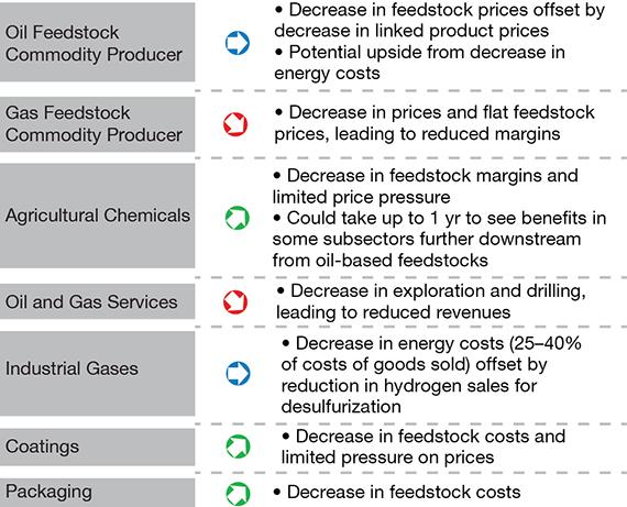
▲Figure 1. Reduced oil prices have impacted sectors of the chemical industry differently.

The sharp decline in oil prices that began in the summer of 2014 — a drop of more than 60%, from over $100/bbl to less than $40/bbl in December 2015 — is having a profound effect on the chemical industry. Unlike other industries that depend on oil solely for energy, the chemical industry also uses oil as feedstock. Furthermore, oil price volatility affects each sector of the chemical industry differently (Figure 1). Some have benefited: Specialty chemical producers, for example, saw feedstock costs drop, yet have often been able to maintain price levels. Others have not: Commodity chemical makers have saved on feedstock and energy, but many have had to pass those savings on to customers.

The fall of crude oil prices is simply the most recent example of major changes to energy and feedstock pricing. Particularly in North America, prices for natural gas, ethane, and, more recently, propane have also dramatically declined.

Regardless of whether lower-cost inputs have helped or hurt, the sudden shifts have served as acute reminders of the need for chemical companies to better manage their businesses amidst an increasingly volatile price environment. Many are finding it hard enough to create near-term, three-year financial forecasts or even land their operating budgets for the coming year. And, evaluating the economic viability of long-term major capital projects has become incredibly difficult.

This article discusses the reasons for the drop in energy and feedstock prices, where the prices could go next, and how price volatility has affected chemical producers. It examines how chemical producers can use scenario planning to prepare for uncertainty, and offers several specific strategic and tactical steps that companies should be taking to position themselves for the eventual correction in oil prices.

The numbers behind the oil price tumble

Trends in production and consumption leading up to the decline explain the sharp drop in oil prices.

Global oil production grew by 5.2 million bbl/day from 2009 to 2013, according to the Energy Information Administration (EIA) (1). Roughly 4 million bbl/day of that increase came from the U.S. and Canada, while the rest of the world contributed 1.2 million bbl/day. During the same period, global oil consumption increased by 6.2 million bbl/day. Thus, North America’s tight oil boom was offset by anemic production in the rest of the world, and consumption that outpaced production masked an impending structural oversupply.

From September 2013 to September 2014, net global production increased by 3 million bbl/day, eclipsing consumption, which grew by only 0.8 million bbl/day. Sustained production in the U.S. and Canada, plus a resurgence of production in Iraq, Libya, and Iran, are responsible for the increase during this time period. In the summer of 2014, the International Energy Agency (IEA) revised downward its 2015 forecast for global oil demand by about 400,000 bbl/day — implying that increased production would not be needed to balance the market in 2015.

Despite IEA’s revised forecast, oil prices still hovered at about $95/bbl in September 2014, which shows the difficulty in predicting short-term market outcomes even with well-known variables. In November 2014, as production continued unabated and Saudi Arabia declined to shoulder the lion’s share of any cuts by the Organization of the Petroleum Exporting Countries (OPEC), the bottom fell out. Within three weeks of OPEC’s Nov. 27, 2014 meeting in Vienna, the benchmark price for Brent crude fell to $60/bbl. (Brent crude and West Texas Intermediate [WTI] are well-known benchmarks for global oil pricing. Brent prices are often higher than WTI prices.)

By late summer 2015, crude oil prices had continued to drop, reaching as low as $40/bbl before rebounding to about $48/bbl in September. The structural elements of the market are in place to continue to produce an oversupply of oil, exerting downward pressure on prices. As producers continue to pump oil to maintain their own revenues, the global picture remains one of oversupply — an indication that prices are not likely to rebound anytime soon.

Oil price recovery scenarios

Executives across a wide range of industries, particularly those most affected by energy prices, are closely watching developments in key locations, from the shale fields of North America to the Geneva meeting rooms of OPEC, to see how production volumes might shift.

The shape of the recovery curve for oil prices hinges on one demand variable and four supply variables:

Consumption growth. China’s slowing growth and Europe’s sluggish economy will likely continue to hinder global oil consumption over the next few years. While the range of forecasts has narrowed considerably, small differences in demand projections can have a large impact on chemical markets and should be taken into account in the near term.

Production from low-cost sources. Bain forecasts oil production by OPEC in 2020 to be 26–40 million bbl/day, with the most likely range being 34–35 million bbl/day — which is more than the current production of about 31 million bbl/day. This increase in low-cost supply will flatten the supply curve, allowing more demand to be fulfilled by lower-cost sources and putting economic pressure on high-cost sources of oil, particularly oil from deep water, Canadian oil sands, and Venezuelan heavy crude oil. High-cost sources will continue to produce in the short term (next 1–2 yr), because the marginal costs of production are still lower than current market prices, but new, high-cost production could face difficulties finding fresh capital.

Committed capital projects. High-cost projects, like deepwater rigs, can take years and billions of dollars to complete; thus, oil producers calculate their breakeven projections based on long-range price predictions. Capital continues to flow to many projects that are already underway, even if their fully loaded costs fall below current market prices. Deepwater projects will continue to add supply for the foreseeable future.

Inventory. With crude oil supplies of countries in the Organisation for Economic Co-operation and Development (OECD) at their highest levels since recordkeeping began, the industry must count this inventory as a short-term supply source. In the U.S., inventory is approaching physical limits that could, if breached, cause WTI prices to plummet to new lows. Supply and demand scenarios for the near term must take into account record-high inventories.

U.S. tight oil. Tight oil is crude oil from shale or another low-permeability geologic formation. Tight oil’s unique characteristics make it one of the few resources that could react quickly to changing conditions.

• It can be ramped up quickly. New wells take only a few weeks and millions of dollars, as opposed to years and billions of dollars, to drill, and they can be drilled and held in reserve.
• It can be shut off quickly. Depletion curves, which show the decrease in production of tight oil wells, are very steep, and first-year decline rates of 60–70% are the norm.
• Breakeven costs vary widely. The breakeven costs of tight oil are typically in the range of $30–$80/bbl. Using assembly-line methods for drilling large numbers of wells at unconventional sources helps bring most production in under $60/bbl, and the costs continue to decline.

Under a scenario in which OPEC produces at new record highs and economics inhibit new capital investment in the highest-cost supply sources, U.S. tight oil could become the marginal production barrel (i.e., the most expensive oil that will still be profitable to sell) and price-setting yardstick.

How volatility affects chemical producers

For chemical producers, price volatility extends well beyond oil, to other energy and feedstock sources.

Ethane (C2). The abundance of low-cost natural gas in North America, often provided by wet shale gas deposits rich in natural gas liquids (NGLs; i.e., ethane, propane, and butanes), drove ethane prices down to gas-equivalent pricing starting in late 2011.

---

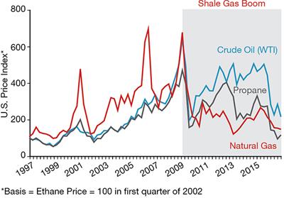
▲Figure 2. The price of propane has recently decoupled from the price of oil. Source: (2–4).

Propane (C3). Similarly, propane broke its historical linkage to the price of oil in 2015 (Figure 2), and in an extreme case actually became negative for western Canadian producers in June 2015 when the costs to separate propane from the natural gas stream to meet local heat-content regulations exceeded the market price.

The potential for sustained low C3 prices has created significant interest within the propane supply chain and has fueled pursuit of major projects. For example, instead of manufacturing propylene as a co-product of naphtha cracking or as a byproduct of petroleum refining, some companies are investing in propane dehydrogenation facilities for on-purpose propylene production. Yet the uncertainty and volatility of future propane prices, as well as ethane and oil prices, remain key factors as chemical producers consider greenfield or brownfield expansions, forecast their medium- and long-term financials, and consider changes to their energy and feedstock slates.

These movements in oil, gas, and other feedstock and energy prices affect chemical markets around the globe in interesting ways.

Scenarios to Deal with Price Volatility

Planning around a single view of the future is a recipe for value destruction. A more strategic approach to planning begins by defining scenarios and then refining the data continually while monitoring signposts that indicate market directions.

The dynamics shaping the energy ecosystem can be thought of along three major supply vectors: natural gas, crude oil, and renewables. For each of these fuel sources, permutations of supply levels create eight plausible scenarios (at the corners of the figure), each of which affects the price of oil and natural gas in different ways.

Inter-fuel substitutions (i.e., substitution between fuel types, such as natural gas for coal) and intra-fuel substitutions (i.e., substitution within fuel types, such as shale gas for coal-bed methane) change the energy mix across the scenarios. Within each scenario, costs decline as operators develop more experience in production for each type of fuel (and, indeed, for each location they produce in). As their costs decline, producers are able to deliver supply at lower prices, and this can alter the supply curve, encouraging substitution of lower-cost fuels for higher-cost ones.

We can track and anticipate the oil and gas industry’s evolution by identifying signposts, such as increases and decreases in U.S. tight oil production, and leading indicators, like the evolving shape of the tight oil supply curve in North America.

---

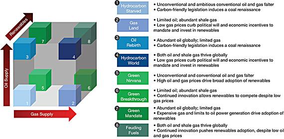
▲ The energy ecosystem can be represented by eight scenarios, depending on supply and experience curve levels for three primary sources of energy.

In the long run, changes in energy mix, more than differences in long-term forecasts for total energy demand, drive demand for any given primary fuel. Since changes in the energy mix result from changes in supply dynamics, a supply-side model is most appropriate. However, as we saw in this most recent downturn, changes in short-term demand forecasts can exacerbate supply-demand imbalances, so planners must build demand considerations into their short-term scenarios.

Differences by product category

Oil prices affect specific chemical products differently, depending on the combined effect of five variables.

Feedstock and energy prices. Some feedstock prices, including those of ethylene and propylene, correlate directly with oil prices, whereas other byproducts of naphtha cracking (e.g., C4 and C5) do not. Energy-intensive processes, such as the chlor-alkali process for making chlorine and sodium hydroxide, benefit from lower production costs when their energy prices are linked to oil. Alternative feedstocks, such as those from agricultural products, are now less attractive, as are methanol-to-olefin and coal-to-olefin projects.

Product prices. In an efficient market, the marginal-cost producers determine a product’s price, which is set so that the highest-cost marginal producer generates a profit. In the case of many ethane- and propane-based products, the marginal production is still based on naphtha cracking; as a result, prices are correlated to naphtha and therefore oil. Farther down the value chain, prices for many specialty products (e.g., specialty coatings) are less affected and producers could benefit from a lag in oil price adjustments.

Macro demand. Lower oil prices can contribute to economic growth by encouraging consumption, and, in general, demand is easier to predict than supply. The longer oil prices remain low, the larger the effect. Economists estimate that the net effect of a $40/bbl reduction in oil prices in 2014 will be an increase in global gross domestic product (GDP) of 0.5–0.6% in 2015 and 1.4–1.6% in 2016. Yet the direct benefits of lower oil prices are partially offset by negative factors, including concerns about deflation.

Product demand. Volatile oil prices first and foremost impact GDP. Because most chemical demand growth is linked to GDP, there is a direct effect on all product categories. Yet the variation at the individual product level can be much more pronounced, depending on the substitution potential (good or bad) and the dynamics of the end-market application. A Bain study concluded that the demand for one bio-based polymer drops off sharply when its price is more than 10% higher than the price of petroleum-based alternatives.

Oil prices also impact the demand for batteries for electric vehicles. Lower oil prices make electric vehicles relatively more expensive to own, and reduced demand (and the second-order effect on the rate of technology development) may delay the adoption of electric vehicles by a few years.

Indirect costs. Capital cost inflation in the chemical industry during the 2011–2014 time period was about 10%, and this was reflected in equipment prices, contractor support costs, and other costs. Most oil companies have now deferred or canceled some capital projects and are working to reduce operating costs. This has reduced the cost per unit of skilled labor, and is likely to also reduce capital costs for chemical companies that rely on the same suppliers.

Differences by geography

Volatile oil prices have affected North American and European chemical producers differently.

North America. While the direct effects of shale gas production have been largely confined to North American markets, the drop in oil prices has impacted markets around the world, although the effect varies by region. In North America, the oil-to-gas price ratio averaged 17 to 1 during the first quarter of 2015. Many projects along the Gulf of Mexico base their business cases on the oil-to-gas spread, which has changed dramatically. A joint venture between U.S.-based Axiall and Lotte Chemical of Korea has delayed construction of an ethane cracker in Louisiana because of uncertainty in energy markets. In January 2015, Sasol announced it would delay a final investment decision on its proposed large gas-to-liquids project in the U.S. to conserve cash in response to lower international oil prices.

North America remains a very attractive location for producing chemicals, particularly those based on ethane and those that require large amounts of energy to manufacture. If all of the announced ethane-based ethylene capacity expansions were built, North America’s cracker capacity would increase by about 40% by early 2020. Several of those announced projects are already being delayed or cancelled as companies wrestle with the economics and the range of uncertainty in product prices, feedstock costs, and capital costs.

We believe that under most scenarios, ethane pricing will remain closely linked to natural gas prices, rather than oil prices. Market prices on the U.S. Gulf Coast will be set by the natural gas price plus the cost of transport of marginal supply, processing, and fractionation.

Sustained low oil prices will reduce profits for some U.S. petrochemical producers below recent peaks, but in many cases, profits will remain above their average historic rates at least for the next few years. Even if oil prices recover over the next three to five years, any increases will likely be partially offset by increased production capacity.

Europe. European chemical producers are still at a cost disadvantage compared with producers in North America, due primarily to the higher costs of natural gas and electricity in Europe. However, the gap has narrowed.

---

---

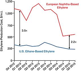
▲Figure 3. European production costs of naphtha-based ethylene have dropped considerably since 2013 (top), narrowing the cost advantage of U.S. ethane-based ethylene production (bottom). Source: Nexant.

Ethylene production costs in Europe were 3.5 times higher than costs in America in the fourth quarter of 2012. Two years later, they had fallen to only 2.2 times higher (Figure 3).

European gas prices remain approximately 2.5 times higher than those in the U.S. Gas prices in Europe do not reflect the cost of gas supply, and the region requires significant import volumes to meet demand. High prices for power raise the costs of all chemicals, but some segments will see a particularly significant increase — e.g., chlor-alkali and soda ash, which are energy intensive to produce.

The effect of lower oil prices also varies at the national level. For instance, countries that depend heavily on oil, like Russia, are likely to see a drop in GDP.

Movement in foreign exchange rates is a compounding factor. The strength of the dollar creates new challenges for U.S. crackers that export to Asia and Latin America. The drop in the value of the euro relative to the dollar is bad news for companies that buy in dollars and sell in euros.

Strategic responses for chemical producers

No one knows when or how oil prices will change in the future, and the industry’s leaders must form their short- and medium-term strategies amid great uncertainty. However, here are some strategies to consider when charting a course through the oil storm.

“No regrets” actions deliver benefits under current and future price scenarios. The most important action is reducing costs. Now is the time to enlist the entire organization to help reduce general and administrative costs to create a leaner organization. Tightening supply chains and increasing manufacturing efficiency will also help, as will renegotiating long-term feedstock contracts for both ethane (due to plentiful supply) and naphtha. With feedstock prices low, look for ways to actively manage the spread between low feedstock costs and product selling prices in order to maintain profit margins as long as possible. Innovation and differentiation also help increase price resilience.

Hold the line on operational excellence. On the other hand, take care not to cut too deeply and risk setting back operational excellence programs put in place to address the inherent risks in operations in a cost-effective and transparent way. Short-term cost cuts may deliver immediate relief, but the wrong cuts can threaten the balance of safety, reliability, and the ability to serve customers. In previous economic downturns, companies that reduced costs by cutting corners on maintenance or by releasing valuable talent paid for it later. Executives looking for savings in the current low-price environment must be thoughtful in making these decisions.

Structural reforms to improve growth and profitability include aggressive operational or commercial actions designed to improve a producer’s position or capture new market opportunities. Looking 20 years out, North America remains attractive for investment. Subject to affordability, this could be an ideal time to push projects forward. The slowdown in upstream capital investment has led to lower costs, and engineering and craft labor are now more readily available than they were two years ago. However, feedstock (and product) prices could be quite different by the time new assets come online.

Conversely, European producers should focus on making the industry more resilient to be better prepared for future oil price increases. One strategy is to invest in facilities to import U.S. feedstock. SABIC is converting its Wilton cracker in the U.K. from naphtha to U.S. ethane, and completion is planned for 2016. This follows similar investments by INEOS at Grangemouth in Scotland and Borealis at Stenungsund in Sweden. Such moves are complex and involve parallel investment in pipelines and NGL separation facilities in North America, either directly or through partnerships.

Other strategies include consolidating through mergers or acquisitions to reinforce existing positions, retiring uncompetitive assets, and reducing overcapacity while preserving the cost savings afforded by a large scale. Examples include BASF’s 2005 sale of its polystyrene assets to INEOS and the 2014 merger of the chlorovinyls assets of INEOS and Solvay to form INOVYN.

European executives should also work with regulators to advocate for more integrated energy policies and for tax structures that encourage research and development (R&D) and other investments in the industry.

Selective big bets radically reshape portfolios to refocus investment or take advantage of new opportunities. Some large chemical companies are spinning off non-core assets to focus their investments, while others are making significant investments in R&D or mergers and acquisitions as they seek out a new competitive advantage.

Short-term tactics

Practically speaking, three immediate priorities emerge.

Reduce costs. This is even more important in a volatile market. Cutting operating expenses and embracing a philosophy focused on lowest unit cost is critical to generating cash consistently through the market and margin cycle underway.

Design for feedstock flexibility. Although this provides options, it also increases costs. The ideal setup is an asset portfolio dominated by simple, low-cost assets (e.g., ethane-based crackers in the ethylene chain) with a smaller allocation to flexible assets and alternative process routes, such as propane dehydrogenation (PDH) and methanol-to-olefins (MTO). Assembling an asset portfolio like this is easier for larger companies, but smaller companies can develop partnerships that give them options.

Consider integration (horizontal and vertical). When done correctly, this can diversify end-market exposure across different cycles and generate profit from a wider market base.

Closing thoughts

Uncertainty in the oil market has fundamental implications for the way companies think about investments. Traditional accounting appraisal tools, such as net present value and internal rate of return, combined with analysis of the sensitivity to input assumptions, are of limited use when the investments themselves are inherently uncertain. The most successful and adaptable approach is to develop a range of credible but extreme scenarios, including black swan events, to evaluate alternative strategies

When a market’s future is unclear and the upside of a successful investment outweighs the downside of an unsuccessful one, the best investment approach is to build a diversified portfolio of products and businesses. As in capital markets, some investments will fail while others will pay back handsome returns. Uncertainty benefits larger, well-funded companies that can more easily diversify risk across a portfolio of investments.

The effects of lower oil prices on chemical producers are complex, benefiting some while hurting others. Over time, the industry will see more profound effects as companies shift production to lower-cost regions and seek to reinvent themselves and restructure the industry. As always, the winners will be those that take advantage of the opportunities created.

Literature Cited

1. U.S. Energy Information Administration, “International Energy Statistics,” EIA, Washington, DC, www.eia.gov/cfapps/ipdbproject/iedindex3.cfm?tid=5&pid=53&aid=1&cid=ww,&syid=2009&eyid=2013&unit=TBPD (accessed Nov. 2015).
2. U.S. Energy Information Administration, “Cushing, OK WTI Spot Price FOB,” www.eia.gov/dnav/pet/hist/LeafHandler.ashx?n=pet&s=rwtc&f=m (accessed Nov. 2015).
3. U.S. Energy Information Administration, “Henry Hub Natural Gas Spot Price,” www.eia.gov/dnav/ng/hist/rngwhhdM.htm (accessed Nov. 2015).
4. U.S. Energy Information Administration, “Mont Belvieu, TX Propane Spot Price FOB,” www.eia.gov/dnav/pet/hist/LeafHandler.ashx?n=pet&s=eer_epllpa_pf4_y44mb_dpg&f=m (accessed Nov. 2015).

---