Introduction to Deep Learning: Part 1

Although deep learning, a branch of artificial intelligence, has become prominent only recently, it is based on concepts that are familiar to chemical engineers. This article describes artificial neural networks — the algorithms that enable deep learning.

The ancient Chinese game of Go has more possible moves than the number of atoms in the universe. Unlike chess, Go cannot be won using brute-force computing power to analyze a lot of moves — there are just too many possibilities. And, unlike chess, strategies for winning Go cannot be meaningfully codified by rules: its principles are mysterious. In some cultures, Go is seen as a way for humans to connect with the divine via instances of intuition, by “knowing without knowing how you know.”

Experts believed that computers would not be able to defeat top human players at Go for decades, if ever. But in 2016, a computer program called AlphaGo defeated Lee Sedol, the legendary world champion of Go (1). During the games, AlphaGo played highly inventively, making moves that no human ever would, and defeated the 18-time world champion four games to one.

AlphaGo is an artificial intelligence (AI) program built using deep learning technologies. From self-driving cars to lawyer-bots (2), deep learning is fueling what many believe will be the biggest technology revolution the world has seen. “Just as electricity transformed almost everything 100 years ago, I actually have a hard time thinking of an industry that I don’t think AI will transform in the next several years,” says Andrew Ng, who has held positions as Director of the Stanford AI Lab, Chief Scientist of Baidu, and Founder of Google Brain.

Chemical engineers routinely use computers for modeling, simulation, design, and optimization of chemical processes. Typically, the computational methods are numerical algorithms (i.e., regression, statistics, differential equations, etc.) performed with software tools like Excel, MatLab, AspenPlus, CHEMCAD, COMSOL Multiphysics, etc. All of these methods and tools are applications of well-known chemical engineering principles, which the engineer combines and applies intelligently to solve high-level problems. Could computers do more than mere computation and someday solve high-level problems like a chemical engineer?

“The vision is that you’ll be able to walk up to a system and say, ‘I want to make this molecule.’ The software will tell you the route you should make it from, and the machine will make it,” says Klavs Jensen, the Warren K. Lewis Professor of Chemical Engineering at MIT (3). His research uses deep learning to identify a pathway to transform a set of available reactants into a target compound (4). Outside academia, deep learning is already being used by practicing engineers to solve a whole range of previously intractable problems and may become as valuable as Excel to chemical engineers in the future.

What is deep learning?

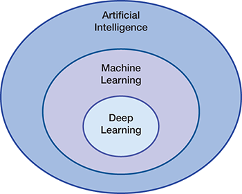
▲Figure 1. Machine learning is a branch of artificial intelligence that gives computers the ability to learn without being programmed. Deep learning is a subfield of machine learning.

Artificial intelligence is the capability of a machine to imitate intelligent human behavior (Figure 1). Machine learning (ML) is a branch of AI that gives computers the ability to “learn” — often from data — without being explicitly programmed. Deep learning is a subfield of ML that uses algorithms called artificial neural networks (ANNs), which are inspired by the structure and function of the brain and are capable of self-learning. ANNs are trained to “learn” models and patterns rather than being explicitly told how to solve a problem.

The building block of an ANN is called the perceptron, which is an algorithm inspired by the biological neuron (5). Although the perceptron was invented in 1957, ANNs remained in obscurity until just recently because they require extensive training, and the amount of training to get useful results exceeded the computer power and data sizes available.

To appreciate the recent increase in computing power, consider that in 2012 the Google Brain project had to use a custom-made computer that consumed 600 kW of electricity and cost around $5,000,000. By 2014, Stanford AI Lab was getting more computing power by using three off-the-shelf graphics processing unit (GPU)-accelerated servers that each cost around $33,000 and consumed just 4 kW of electricity. Today, you can buy a specialized Neural Compute Stick that delivers more than 100 gigaflops of computing performance for $80.

The perceptron

▲Figure 2. A human neuron collects inputs from other neurons using dendrites and sums all the inputs. If the total is greater than a threshold value, it produces an output.

The average human brain has approximately 100 billion neurons. A human neuron uses dendrites to collect inputs from other neurons, adds all the inputs, and if the resulting sum is greater than a threshold, it fires and produces an output. The fired output is then sent to other connected neurons (Figure 2).

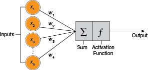
▲Figure 3. A perceptron is a mathematical model of a neuron. It receives weighted inputs, which are added together and passed to an activation function. The activation function decides whether it should produce an output.

A perceptron is a mathematical model of a biological neuron (6). Just like a real neuron, it receives inputs and computes an output. Each input has an associated weight. All the inputs are individually multiplied by their weights, added together, and passed into an activation function that determines whether the neuron should fire and produce an output (Figure 3).

There are many different types of activation functions with different properties, but one of the simplest is the step function (7). A step function outputs a 1 if the input is higher than a certain threshold, otherwise it outputs a 0. For example, if a perceptron has two inputs (x₁ and x₂):

x₁ = 0.9

x₂ = 0.7

which have weightings (w₁ and w₂) of:

w₁ = 0.2

w₂ = 0.9

and the activation function threshold is equal to 0.75, then weighing the inputs and adding them together yields:

x₁w₁ + x₂w₂ = (0.9×0.7) + (0.2×0.9) = 0.81

Because the total input is higher than the threshold (0.75), the neuron will fire. Since we chose a simple step function, the output would be 1.

So how does all this lead to intelligence? It starts with the ability to learn something simple through training.

Training a perceptron

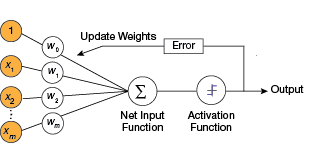
▲Figure 4. To train a perceptron, the weights are adjusted to minimize the output error. Output error is defined as the difference between the desired output and the actual output.

Training a perceptron involves feeding it multiple training samples and calculating the output for each of them. After each sample, the weights are adjusted to minimize the output error, usually defined as the difference between the desired (target) and the actual outputs (Figure 4).

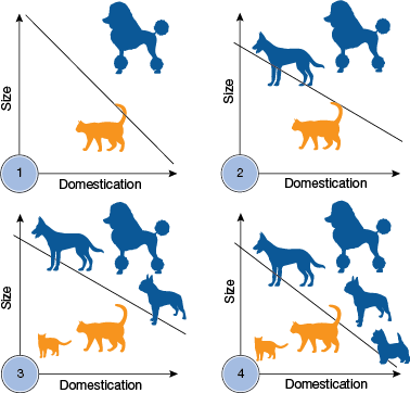
▲Figure 5. A perceptron can learn to separate dogs and cats given size and domestication data. As more training examples are added, the perceptron updates its linear boundary.

By following this simple training algorithm to update weights, a perceptron can learn to perform binary linear classification. For example, it can learn to separate dogs from cats given size and domestication data, if the data are linearly classifiable (Figure 5).

The perceptron’s ability to learn classification is significant because classification underlies many acts of intelligence. A common example of classification is detecting spam emails. Given a training dataset of spam-like emails labeled as “spam” and regular emails labeled as “not-spam,” an algorithm that can learn characteristics of spam emails would be very useful. Similarly, such algorithms could learn to classify tumors as cancerous or benign, learn your music preferences and classify songs as “likely-to-like” and “unlikely-to-like,” or learn to distinguish normally behaving valves from abnormally behaving valves (8).

Perceptrons are powerful classifiers. However, individually they can only learn linearly classifiable patterns and are unable to handle nonlinear or more complicated patterns.

Multilayer perceptrons

A single neuron is capable of learning simple patterns, but when many neurons are connected together, their abilities increase dramatically. Each of the 100 billion neurons in the human brain has, on average, 7,000 connections to other neurons. It has been estimated that the brain of a three-year-old child has about one quadrillion connections between neurons. And, theoretically, there are more possible neural connections in the brain than there are atoms in the universe.

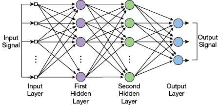
▲Figure 6. A multilayer perceptron has multiple layers of neurons between the input and output. Each neuron’s output is connected to every neuron in the next layer.

A multilayer perceptron (MLP) is an artificial neural network with multiple layers of neurons between input and output. MLPs are also called feedforward neural networks. Feedforward means that data flow in one direction from the input to the output layer. Typically, every neuron’s output is connected to every neuron in the next layer. Layers that come between the input and output layers are referred to as hidden layers (Figure 6).

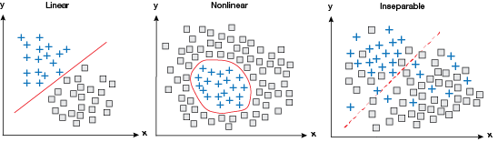
▲Figure 7. Although single perceptrons can learn to classify linear patterns, they are unable to handle nonlinear or other more complicated datasets. Multilayer perceptrons are more capable of handling nonlinear patterns, and can even classify inseparable data.

MLPs are widely used for pattern classification, recognition, prediction, and approximation, and can learn complicated patterns that are not separable using linear or other easily articulated curves. The capacity of an MLP network to learn complicated patterns increases with the number of neurons and layers (Figure 7).

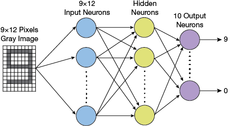
▲Figure 8. A multilayer perceptron for recognizing digits printed on a check would have a grid of inputs to read individual pixels of digits, followed by one or more layers of hidden neurons, and 10 output neurons to indicate which number was recognized.

MLPs have been successful at a wide range of AI tasks, from speech recognition (9) to predicting thermal conductivity of aqueous electrolyte solutions (10) and controlling a continuous stirred-tank reactor (11). For example, an MLP for recognizing printed digits (e.g., the account and routing number printed on a check) would be comprised of a grid of inputs to read individual pixels of digits (say, a 9×12 bitmap), followed by one or more hidden layers, and finally 10 output neurons to indicate which number was recognized in the input (0–9) (Figure 8).

Such an MLP for recognizing digits would typically be trained by showing it images of digits and telling it whether it recognized them correctly or not. Initially, the MLP’s output would be random, but as it is trained, it will adjust weights between the neurons and start classifying inputs correctly.

A typical real-life MLP for recognizing handwritten digits consists of 784 perceptrons that accept inputs from a 28×28 pixel bitmap representing a handwritten digit, 15 neurons in the hidden layer, and 10 output neurons (12). Typically, such an MLP is trained using a pool of 50,000 labeled images of handwritten digits. It can learn to recognize previously unseen handwritten digits with 95% accuracy after a few minutes of training on a well-configured computer.

In a similar fashion, others have used data from Perry’s Chemical Engineers’ Handbook to train an MLP to predict viscosity of a compound (13). In another study, scientists were able to detect faults in a heat exchanger by training an MLP to recognize deviations in temperature and flowrate as symptoms of tube plugging and partial fouling in the heat exchanger internals (14).

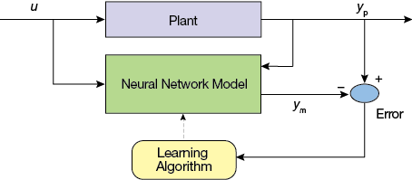
▲Figure 9. An MLP can learn the dynamics of the plant by evaluating the error between the actual plant output and the neural network output.

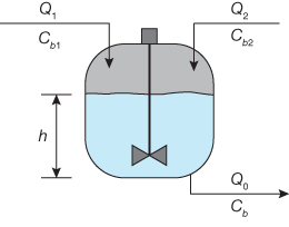
▲Figure 10. A continuous stirred-tank reactor can be trained to maintain appropriate product concentration and flow by using past data about inflow, concentration, liquid level, and outflow.

As another example, MLPs have been used for predictive control of chemical reactors (15). The typical setup trains a neural network to learn the forward dynamics of the plant. The prediction error between the plant output and the neural network output is used for training the neural network (Figure 9). The neural network learns from previous inputs and outputs to predict future values of the plant output. For example, a controller for a catalytic continuous stirred-tank reactor (Figure 10) can be trained to maintain appropriate product concentration and flow by using past data about inflow Q₁ and Q₂ at concentrations C_b1 and C_b2, respectively, liquid level h, and outflow Q₀ at concentration C_b.

In general, given a statistically relevant dataset, an artificial neural network can learn from it (16).

Training a multilayer perceptron

Training a single perceptron is easy — all weights are adjusted repeatedly until the output matches the expected value for all training data. For a single perceptron, weights can be adjusted using the formulas:

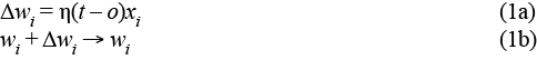
where w_i is the weight, Δw_i is the weight adjustment, t is the target output, o is the actual output, and η is the learning rate — usually a small value used to moderate the rate of change of weights.

However, this approach of tweaking each weight independently does not work for an MLP because each neuron’s output is an input for all neurons in the next layer. Tweaking the weight on one connection impacts not only the neuron it propagates to directly, but also all of the neurons in the following layers as well, and thus affects all the outputs. Therefore, you cannot obtain the best set of weights by optimizing one weight at a time. Instead, the entire space of possible weight combinations must be searched simultaneously. The primary method for doing this relies on a technique called gradient descent.

Imagine you are at the top of a hill and you need to get to the bottom of the hill in the quickest way possible. One approach could be to look in every direction to see which way has the steepest grade, and then step in that direction. If you repeat this process, you will gradually go farther and farther downhill. That is how gradient descent works: If you can define a function over all weights that reflects the difference between the desired output and calculated output, then the function will be lowest (i.e., the bottom of the hill) when the MLP’s output matches the desired output. Moving toward this lowest value will become a matter of calculating the gradient (or derivative of the function) and taking a small step in the direction of the gradient.

Backpropagation, short for “backward propagation of errors,” is the most commonly used algorithm for training MLPs using gradient descent. The backward part of the name stems from the fact that calculation of the gradient proceeds backward through the network. The gradient of the final layer of weights is calculated first and the gradient of the first layer of weights is calculated last.

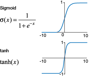
▲Figure 11. Sigmoid and tanh functions are nonlinear activation functions. The output of the sigmoid function is a value between 0 and 1. The output of the sigmoid function can be used to represent a probability, often the probability that the input belongs to a category (e.g., cat or dog).

Before looking at how backpropagation works, recall that a perceptron calculates a weighted sum of its input and then decides whether it should fire. The decision about whether or not to fire is made by the activation function. In the perceptron example, we used a step function that outputted a 1 if the input was higher than a certain threshold, otherwise it out-putted a 0. In practice, ANNs use nonlinear activation functions like the sigmoid or tanh functions (Figure 11), at least in part because a simple step function does not lend itself to calculating gradients — its derivative is 0.

The sigmoid function maps its input to the range 0 to 1. You might recall that probabilities, too, are represented by values between 0 and 1. Hence, the output of the sigmoid function can be used to represent a probability — often the probability that the input belongs to a category (e.g., cat or dog). For this reason, it is one of the most widely used activation functions for artificial neural networks.

Example: Training an MLP with backpropagation

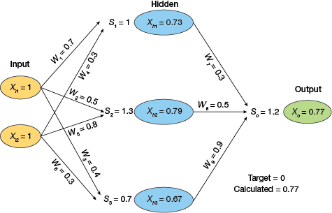
▲Figure 12. An example MLP with three layers accepts an input of [1, 1] and computes an output of 0.77.

Consider a simple MLP with three layers (Figure 12): two neurons in the input layer (X_i1, X_i2) connected to three neurons (X_h1, X_h2, X_h3) in the hidden layer via weights W₁–W₆, which are connected to a single output neuron (X_o) via weights W₇–W₉. Assume that we are using the sigmoid activation function, initial weights are randomly assigned, and input values [1, 1] will lead to an output of 0.77.

Let’s assume that the desired output for inputs [1, 1] is 0. The backpropagation algorithm can be used to adjust weights. First, calculate the error at the last neuron’s (X_o) output:

Recall that the output (0.77) was obtained by applying the sigmoid activation function to the weighted sum of the previous layer’s outputs (1.2):

σ(1.2) = 1/(1 + e^–1.2) = 0.77

The derivative of the sigmoid function represents the gradient or rate of change:

Hence, the gradient or rate of change of the sigmoid function at x = 1.2 is: (0.77) × (1 – 0.77) = 0.177

If we multiply the error in output (–0.77) by this rate of change (0.177) we get –0.13. This can be proposed as a small change in input that could move the system toward the proverbial “bottom of the hill.”

Recall that the sum of the weighted inputs of the output neuron (1.2) is the product of the output of the three neurons in the previous layer and the weights between them and the output neuron:

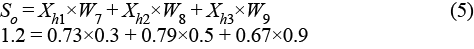
To change this sum (S_o) by –0.13, we can adjust each incoming weight (W₇, W₈, W₉) proportional to the corresponding output of the previous (hidden layer) neuron (X_h1, X_h2, X_h3). So, the weights between the hidden neurons and the output neuron become:

W_7new = W_7old + (–0.13/X_h1) = 0.3 + (–0.13/0.73) = 0.11

W_8new = W_8old + (–0.13/X_h2) = 0.5 + (–0.13/0.79) = 0.33

W_9new = W_9old + (–0.13/X_h3) = 0.9 + (–0.13/0.67) = 0.7

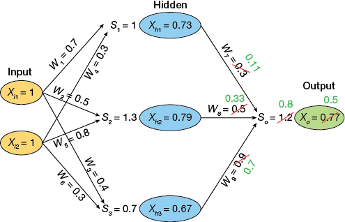
▲Figure 13. A backpropagation algorithm is used to adjust the weightings between the hidden layer neurons and the output neurons, so that the output is closer to the target value (0).

After adjusting the weights between the hidden layer neurons and the output neuron (Figure 13), we repeat the process and similarly adjust the weights between the input and hidden layer neurons. This is done by first calculating the gradient at the input coming into each neuron in the hidden layer. For example, the gradient at X_h3 is: 0.67×(1–0.67) = 0.22.

The proposed change in the sum of weighted inputs of X_h3 (i.e., S₃) can be calculated by multiplying the gradient (0.22) by the proposed change in the sum of weighted inputs of the following neuron (–0.13), and dividing by the weight from this neuron to the following neuron (W₉). Note that we are propagating errors backward, so it was the error in the following neuron (X_o) that we proportionally propagated backward to this neuron’s inputs.

The proposed change in the sum of weighted inputs of X_h3 (i.e., S₃) is:

Change in S₃ = Gradient at X_h3 × Proposed change in S_o/W₉

Change in S₃ = 0.22 × (–0.13)/0.9 = –0.03

Note that we use the original value of W₉ (0.9) rather than the recently calculated new value (0.7) to propagate the error backward. This is because although we are working one step at a time, we are trying to search the entire space of possible weight combinations and change them in the right direction (toward the bottom of the hill). In each iteration, we propagate the output error through original weights, leading to new weights for the iteration. This global backward propagation of the output neuron’s error is the key concept that lets all weights change toward ideal values.

Once you know the proposed change in the weighted sum of inputs of each neuron (S₁, S₂, S₃), you can change the weights leading to the neuron (W₁ through W₆) proportional to the output from the previous neuron. Thus, W₆ changes from 0.3 to 0.27.

Upon repeating this process for all weights, the new output in this example becomes 0.68, which is a little closer to the ideal value (0) than what we started with (0.77). By performing just one such iteration of forward and back propagation, the network is already learning!

A small neural network like the one in this example will typically learn to produce correct outputs after a few hundred such iterations of weight adjustments. On the other hand, training AlphaGo’s neural network, which has tens of thousands of neurons arranged in more than a dozen layers, takes more serious computing power, which is becoming increasingly available.

Looking forward

Even with all the amazing progress in AI, such as self-driving cars, the technology is still very narrow in its accomplishments and far from autonomous. Today, 99% of machine learning requires human work and large amounts of data that need to be normalized and labeled (i.e., this is a dog; this is a cat). And, people need to supply and fine-tune the appropriate algorithms. All of this relies on manual labor.

Other challenges that plague neural networks include:

• Bias. Machine learning is looking for patterns in data. If you start with bad data, you will end up with bad models.
• Over-fitting. In general, a model is typically trained by maximizing its performance on a particular training dataset. The model thus memorizes the training examples, but may not learn to generalize to new situations and datasets.
• Hyper-parameter optimization. The value of a hyper-parameter is defined prior to the commencement of the learning process (e.g., number of layers, number of neurons per layer, type of activation function, initial value of weights, value of the learning rate, etc.). Changing the value of such parameters by a small amount can invoke large changes in the performance of the network.
• Black-box problems. Neural networks are essentially black boxes, and researchers have a hard time understanding how they deduce particular conclusions. Their operation is largely invisible to humans, rendering them unsuitable for domains in which verifying the process is important.

Thus far, we have looked at neural networks that learn from data. This approach is called supervised learning. As discussed in this article, during the training of a neural network under supervised learning, an input is presented to the network and it produces an output that is compared with the desired/target output. An error is generated if there is a difference between the actual output and the target output and the weights are adjusted based on this error until the actual output matches the desired output. Supervised learning relies on manual human labor for collecting, preparing, and labeling a large amount of training data.

In Part 2 of this series, we will delve into two other approaches that are more autonomous: unsupervised learning and reinforcement learning.

Unsupervised learning does not depend on target outputs for learning. Instead, inputs of a similar type are combined to form clusters. When a new input pattern is applied, the neural network gives an output indicating the class to which the input pattern belongs.

Reinforcement learning involves learning by trial and error, solely from rewards or punishments. Such neural networks construct and learn their own knowledge directly from raw inputs, such as vision, without any hand-engineered features or domain heuristics. AlphaGo Zero, the successor to AlphaGo, is based on reinforcement learning. Unlike AlphaGo, which was initially trained on thousands of human games to learn how to play Go, AlphaGo Zero learned to play simply by playing games against itself. Although it began with completely random play, it eventually surpassed human level of play and defeated the previous version of AlphaGo by 100 games to 0.

In Part 2 we will also look at exotic neural network architectures like long short-term memory networks (LSTMs), convolutional neural networks (CNNs), and generative adversarial networks (GANs).

Last but not least, we will discuss social and ethical aspects, as the recent explosion of progress in AI has created fear that it will evolve from being a benefit to human society to taking control. Even Stephen Hawking, who was one of Britain’s most distinguished scientists, warned of AI’s threats. “The development of full artificial intelligence could spell the end of the human race,” said Hawking (17).

Literature Cited

- AlphaGo, “The Story of AlphaGo So Far,” Deepmind, https://deepmind.com/research/alphago/ (accessed May 4, 2018).
- Son, H., “JPMorgan Software Does in Seconds What Took Lawyers 360,000 Hours,” Bloomberg,www.bloomberg.com/news/articles/2017-02-28/jpmorgan-marshals-an-army-of-developers-to-automate-high-finance (Feb. 27, 2017).
- Hardesty, L., “Computer System Predicts Products of Chemical Reactions,” MIT News, MIT News Office, http://news.mit.edu/2017/computer-system-predicts-products-chemical-reactions-0627 (June 27, 2017).
- Coley, C. W., et al., “Prediction of Organic Reaction Outcomes Using Machine Learning,” ACS Central Science,3 (5), pp. 434–443 (Apr. 18, 2017).
- Rosenblatt, F., “The Perceptron: A Probabilistic Model for Information Storage And Organization in the Brain,” Psychological Review,65 (6), www.ling.upenn.edu/courses/cogs501/Rosenblatt1958.pdf (1958).
- Clabaugh, C., et al., “Neural Networks: The Perceptron,” Stanford Univ., https://cs.stanford.edu/people/eroberts/courses/soco/projects/neural-networks/Neuron/index.html (accessed May 4, 2018).
- Sharma, A. V, “Understanding Activation Functions in Neural Networks,” Medium, https://medium.com/the-theory-of-everything/understanding-activation-functions-in-neural-networks-9491262884e0 (Mar. 30, 2017).
- Pandya, D., et al., “Digital Twins for Predicting Early Onset of Failures Flow Valves,” presented at the AIChE Spring Meeting and Global Congress on Process Safety, Orlando, FL (Apr. 23, 2018).
- Azzizi, N., and A. Zaatri, “A Learning Process Of Multilayer Perceptron for Speech Recognition,” International Journal of Pure and Applied Mathematics,107 (4), pp. 1005–1012 (May 7, 2016).
- Eslamloueyan, R., et al., “Using a Multilayer Perceptron Network for Thermal Conductivity Prediction of Aqueous Electrolyte Solutions,” Industrial and Engineering Chemistry Research,50 (7), pp. 4050–4056 (Mar. 2, 2011).
- ZareNezhad, B., and A. Aminian, “Application Of The Neural Network-Based Model Predictive Controllers in Nonlinear Industrial Systems. Case Study,” Journal of the Univ. of Chemical Technology and Metallurgy,46 (1), pp. 67–74 (2011).
- Nielsen, M., “Chapter 1: Using Neural Nets to Recognize Handwritten Digits,” in “Neural Networks and Deep Learning,” http://neuralnetworksanddeeplearning.com/chap1.html (Dec. 2017).
- Moghadassi, A., et al., “Application of Artificial Neural Network for Prediction of Liquid Viscosity,” Indian Chemical Engineer,52 (1), pp. 37–48 (Apr. 23, 2010).
- Himmelblau, D. M., et al., “Fault Classification with the AID of Artificial Neural Networks,” IFAC Proceedings Volumes,24 (6), pp. 541–545 (Sept. 1991).
- Vasičkaninová, A., and M. Bakošová, “Neural Network Predictive Control of a Chemical Reactor,” Acta Chimica Slovaca,2 (2), pp. 21–36 (2009).
- Rojas, R., “Chapter 9: Statistics and Neural Networks,” in “Neural Networks: A Systematic Introduction,” Springer-Verlag, Berlin, Germany (1996).
- Cellan-Jones, R., “Stephen Hawking Warns Artificial Intelligence Could End Mankind,” BBC News, www.bbc.com/news/technology-30290540 (Dec. 2, 2014).
Amit Gupta is the Chief Information Officer of the American Institute of Chemical Engineers (AIChE). He is responsible for planning, coordinating, and executing the activities of AIChE’s IT function. He has worked for AIChE for more than 9 years, incrementally assuming responsibilities for web, IT, database, and mobile solutions. Previously, he held positions at Altria and Philip Morris International. Gupta attended Nagpur University (India) and received his BE in computer technology.
1
Copyright Permissions
Would you like to reuse content from CEP Magazine? It’s easy to request permission to reuse content. Simply click here to connect instantly to licensing services, where you can choose from a list of options regarding how you would like to reuse the desired content and complete the transaction.